Hydrodynamics and inundation
The shallow-water equations, their waves, and how a computer solves them
By the end of this chapter you should be able to:
- Explain what inundation modelling predicts and why it is computationally expensive.
- State the assumptions behind the shallow-water equations and say when they hold.
- Write the two-dimensional shallow-water equations in conservative form, and explain each term.
- Estimate the speed of a shallow-water wave, and the time it takes to cross a domain.
- Describe initial and boundary conditions, the lake-at-rest equilibrium, and why wet/dry fronts are difficult.
- Explain how a finite-volume solver works, what numerical diffusion is, and why grid refinement matters.
- Describe the scenario dataset used in the rest of the seminar.
1 Why model inundation?
Inundation is the flooding of normally dry land: by a river overtopping its banks, a storm surge, a tsunami or a dam failure. Planners and emergency managers want to know where the water goes, how deep it gets and how fast it moves. They rarely want one answer. They want many: for different rainfall, different breach locations, different tide levels, or with and without a new levee.
Each answer requires solving a set of partial differential equations (PDEs) over a large area, often for hours of simulated time and on fine grids. A single high-resolution simulation can take minutes to hours. Thousands of them, for an ensemble or a real-time forecast, quickly become impractical.
This is the motivation for the whole seminar. A surrogate (or emulator) is a cheaper model trained to reproduce the expensive one. Before we can judge a surrogate, we need to understand what the expensive model computes. That is the subject of this chapter.
2 The shallow-water idea
Water in a river, an estuary or a flooded street is usually wide and shallow: the flow extends over kilometres horizontally, but only metres vertically. The shallow-water equations (SWE), also called the Saint-Venant equations, exploit this.
Instead of tracking the velocity at every height in the water column, they track only its depth average. The three-dimensional flow is replaced by a two-dimensional one, which is much cheaper to compute.
The averaging rests on three assumptions:
- Long waves. The horizontal length scale \(L\) of the flow features is much larger than the water depth \(H\), so \(H/L \ll 1\).
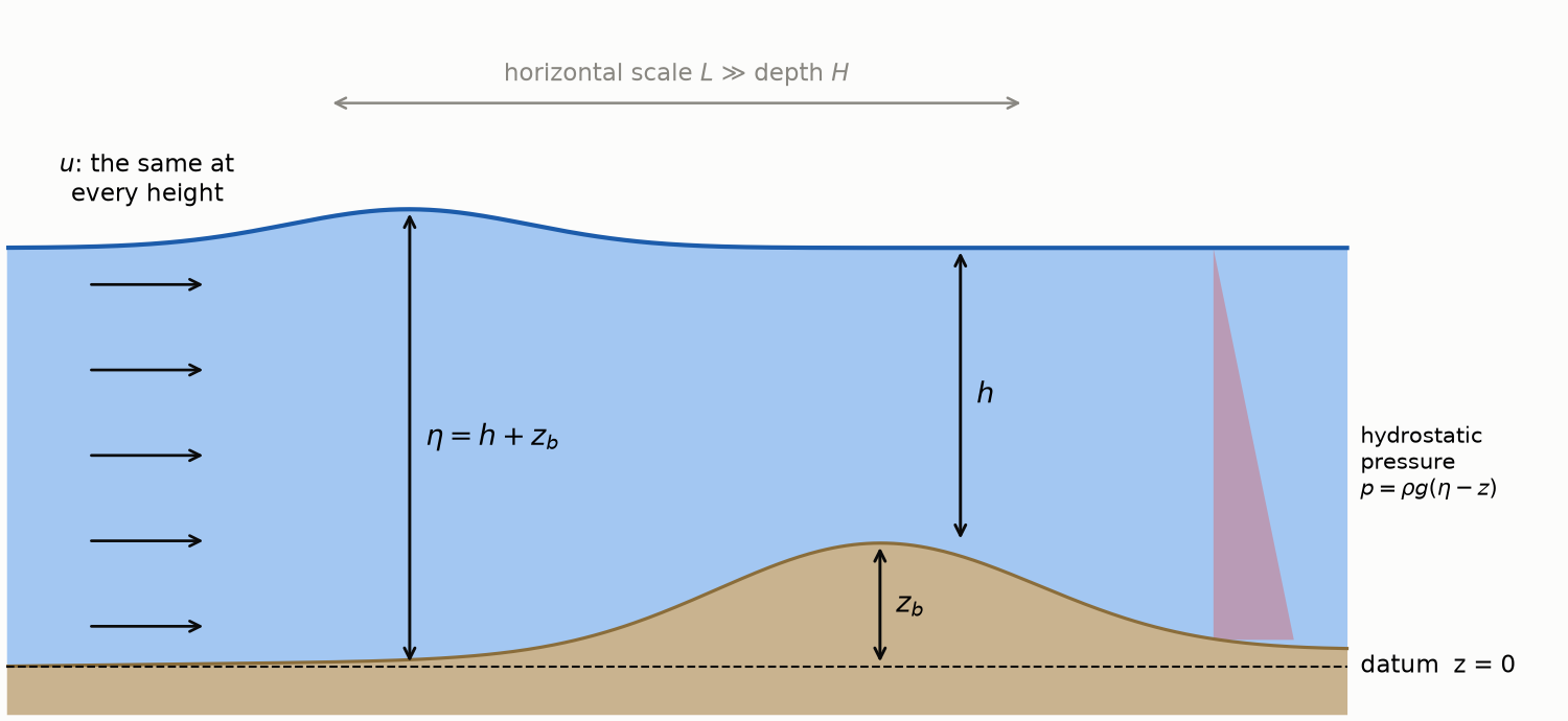
- Hydrostatic pressure. Vertical accelerations are small, so the pressure at a point is just the weight of the water above it: \(p = \rho g (\eta - z)\) at height \(z\) below the free surface \(\eta\), where \(\rho\) is the density of water.
- Vertically uniform velocity. The horizontal velocity hardly varies with height, so its depth average represents it well.
These hold well for tides, floods, storm surges and tsunamis far from the coast. They fail for short, steep wind waves, for breaking waves in detail, and for flows with strong vertical structure.
2.1 Variables and notation
Table 1 lists the quantities used throughout the seminar, and Figure 1 shows how they relate.
| Symbol | Meaning | Unit |
|---|---|---|
| \(x, y\) | Horizontal coordinates | m |
| \(t\) | Time | s |
| \(z_b(x,y)\) | Bed elevation (bathymetry or topography); written \(b\) in some code | m |
| \(h(x,y,t)\) | Water depth, from the bed to the free surface | m |
| \(\eta = h + z_b\) | Free-surface elevation | m |
| \(u, v\) | Depth-averaged velocities in \(x\) and \(y\) | m/s |
| \(q_x = hu,\ q_y = hv\) | Discharges per unit width (volume flux) | m²/s |
| \(g\) | Gravitational acceleration, 9.81 | m/s² |
We work with discharge \(q = hu\) rather than velocity \(u\) because discharge is what the equations conserve, as we see next.
3 Conservation of mass
Consider a fixed rectangle of ground, \(\Delta x\) by \(\Delta y\). The volume of water above it is \(h\,\Delta x\,\Delta y\). That volume changes only if water flows in or out through the four sides. Through the left side, water enters at the rate \(q_x(x)\,\Delta y\); through the right side it leaves at the rate \(q_x(x+\Delta x)\,\Delta y\). Doing the same in \(y\), dividing by \(\Delta x \Delta y\) and letting the rectangle shrink gives
\[ \begin{equation} \frac{\partial h}{\partial t} + \frac{\partial q_x}{\partial x} + \frac{\partial q_y}{\partial y} = 0. \label{eq-mass} \end{equation} \]
In words: depth rises where more water flows in than out. Without rain, infiltration or inflow, Equation \(\eqref{eq-mass}\) guarantees that the total volume \(\iint h\,dx\,dy\) in a walled basin never changes. Any good model, learned or not, should respect this, so we check it in every evaluation.
4 Conservation of momentum
Newton’s second law applied to the same column says that its momentum changes because of momentum carried in and out by the flow, and because of forces.
- Advection. Moving water carries its momentum with it. The flux of \(x\)-momentum through a side normal to \(x\) is \(q_x u = q_x^2/h\).
- Pressure. With hydrostatic pressure, the total pressure force on a vertical face of the column is \(\tfrac12 \rho g h^2\) per unit width. A deeper column on one side pushes water towards the shallower side.
- Bed slope. On a sloping bed, gravity has a component along the slope. It pushes water downhill with a force proportional to \(-g h\, \partial z_b/\partial x\).
Collecting these terms gives the \(x\)-momentum equation, and similarly for \(y\):
\[ \begin{equation} \frac{\partial q_x}{\partial t} + \frac{\partial}{\partial x}\!\left(\frac{q_x^2}{h} + \frac{1}{2} g h^2\right) + \frac{\partial}{\partial y}\!\left(\frac{q_x q_y}{h}\right) = -g h \frac{\partial z_b}{\partial x}, \label{eq-momx} \end{equation} \]
\[ \begin{equation} \frac{\partial q_y}{\partial t} + \frac{\partial}{\partial x}\!\left(\frac{q_x q_y}{h}\right) + \frac{\partial}{\partial y}\!\left(\frac{q_y^2}{h} + \frac{1}{2} g h^2\right) = -g h \frac{\partial z_b}{\partial y}. \label{eq-momy} \end{equation} \]
Real floods also feel bed friction, wind and Coriolis forces. Our benchmark leaves them out to keep the physics clear; they would appear as extra terms on the right-hand side.
4.1 The compact conservative form
Equations \(\eqref{eq-mass}\)–\(\eqref{eq-momy}\) share one structure. Stack the state into a vector \(\mathbf U\) and write
\[ \begin{equation} \frac{\partial \mathbf U}{\partial t} + \frac{\partial \mathbf F(\mathbf U)}{\partial x} + \frac{\partial \mathbf G(\mathbf U)}{\partial y} = \mathbf S(\mathbf U, z_b), \label{eq-conservative} \end{equation} \]
with
\[ \begin{equation} \mathbf U = \begin{pmatrix} h \\ q_x \\ q_y \end{pmatrix},\quad \mathbf F = \begin{pmatrix} q_x \\ q_x^2/h + \tfrac12 g h^2 \\ q_x q_y / h \end{pmatrix},\quad \mathbf G = \begin{pmatrix} q_y \\ q_x q_y/h \\ q_y^2/h + \tfrac12 g h^2 \end{pmatrix},\quad \mathbf S = \begin{pmatrix} 0 \\ -g h\, \partial_x z_b \\ -g h\, \partial_y z_b \end{pmatrix}. \label{eq-fluxes} \end{equation} \]
\(\mathbf F\) and \(\mathbf G\) are fluxes: how much of each conserved quantity crosses a line per unit time. \(\mathbf S\) is a source: what the bed adds or removes locally. This “rate of change + net outflow of flux = source” form is the template for the finite-volume solver below, and for the physics losses in Chapters 2 and 4.
5 Waves: what the equations do
The equations are nonlinear, but much of their behaviour shows up in a simpler, linear version. Suppose the water is nearly at rest over a flat bed with still depth \(H\), so that \(h = H + \eta'\) with a small surface displacement \(\eta'\) and small velocities. Dropping all products of small quantities in Equations \(\eqref{eq-mass}\) and \(\eqref{eq-momx}\) gives
\[ \begin{equation} \frac{\partial \eta'}{\partial t} + H\left(\frac{\partial u}{\partial x} + \frac{\partial v}{\partial y}\right) = 0,\qquad \frac{\partial u}{\partial t} + g\frac{\partial \eta'}{\partial x} = 0,\qquad \frac{\partial v}{\partial t} + g\frac{\partial \eta'}{\partial y} = 0. \label{eq-linear} \end{equation} \]
Differentiating the first equation in time and substituting the other two eliminates the velocities:
\[ \begin{equation} \frac{\partial^2 \eta'}{\partial t^2} = c^2 \left(\frac{\partial^2 \eta'}{\partial x^2} + \frac{\partial^2 \eta'}{\partial y^2}\right), \qquad c = \sqrt{gH}. \label{eq-wave} \end{equation} \]
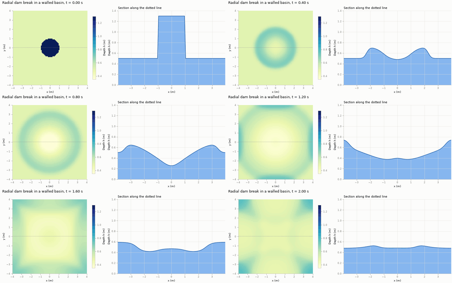
This is the wave equation. A bump in the water surface does not stay put: it collapses and sends out a ring-shaped wave travelling at the shallow-water wave speed \(c = \sqrt{gH}\). The speed depends only on depth. In 1 m of water, \(c \approx 3.1\) m/s; in a 4 km deep ocean, a tsunami travels at about 200 m/s.
Figure 2 shows this in two dimensions. A raised column of water collapses and sends a ring outwards. The ring reflects from the walls, and the reflections cross and interfere.
Two dimensionless numbers tell us how nonlinear a flow is:
- The amplitude ratio \(\varepsilon = a/H\), for a wave of height \(a\). When it is small, Equation \(\eqref{eq-linear}\) is a good approximation.
- The Froude number \(\mathrm{Fr} = |\mathbf u|/\sqrt{gh}\), the flow speed compared with the wave speed. Flows with \(\mathrm{Fr} < 1\) are subcritical (waves can travel upstream). Flows with \(\mathrm{Fr} > 1\) are supercritical, like the fast sheet of water after a dam break.
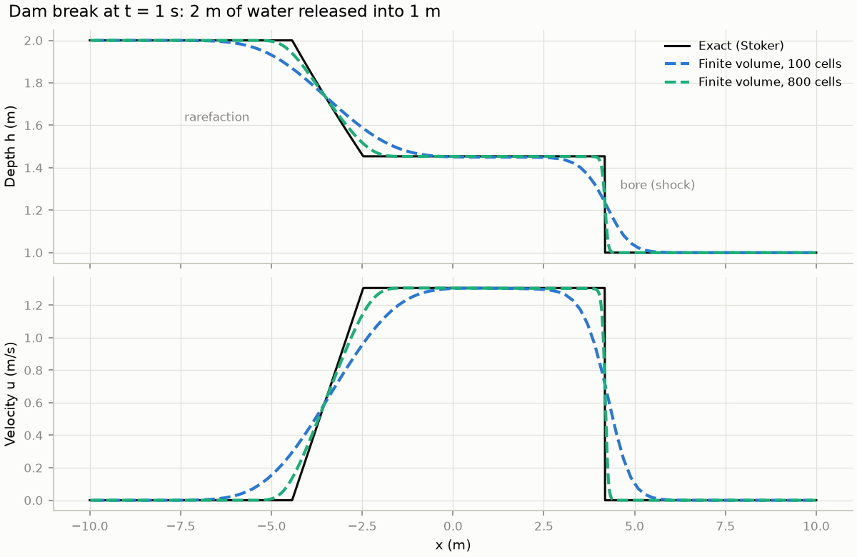
When \(\varepsilon\) is not small, deeper parts of a wave travel faster than shallower ones. The back of the wave catches up with the front, and the wave steepens into a bore, a moving jump in depth. Mathematically a bore is a shock: a discontinuity that the differential form, Equation \(\eqref{eq-conservative}\), cannot describe pointwise, though the integral (conservation) form still can. Figure 3 shows one.
6 Initial and boundary conditions
The PDEs say how the state changes. To get a unique solution we also need where it starts and what happens at the edges.
- Initial condition. The state \(\mathbf U(x,y,0) = (h_0, q_{x,0}, q_{y,0})\) everywhere at \(t=0\), together with the bed \(z_b\). In this seminar, these four fields are exactly the input to the learned models of Chapters 3–5.
- Boundary conditions. Our basin is closed by reflective walls: no water crosses them, so the normal discharge is zero (\(q_x = 0\) on the left and right walls, \(q_y = 0\) on the bottom and top). Waves that reach a wall bounce back. Other common choices are open (outflow) boundaries, which let waves leave, and prescribed inflow, such as a river hydrograph.
6.1 The lake at rest
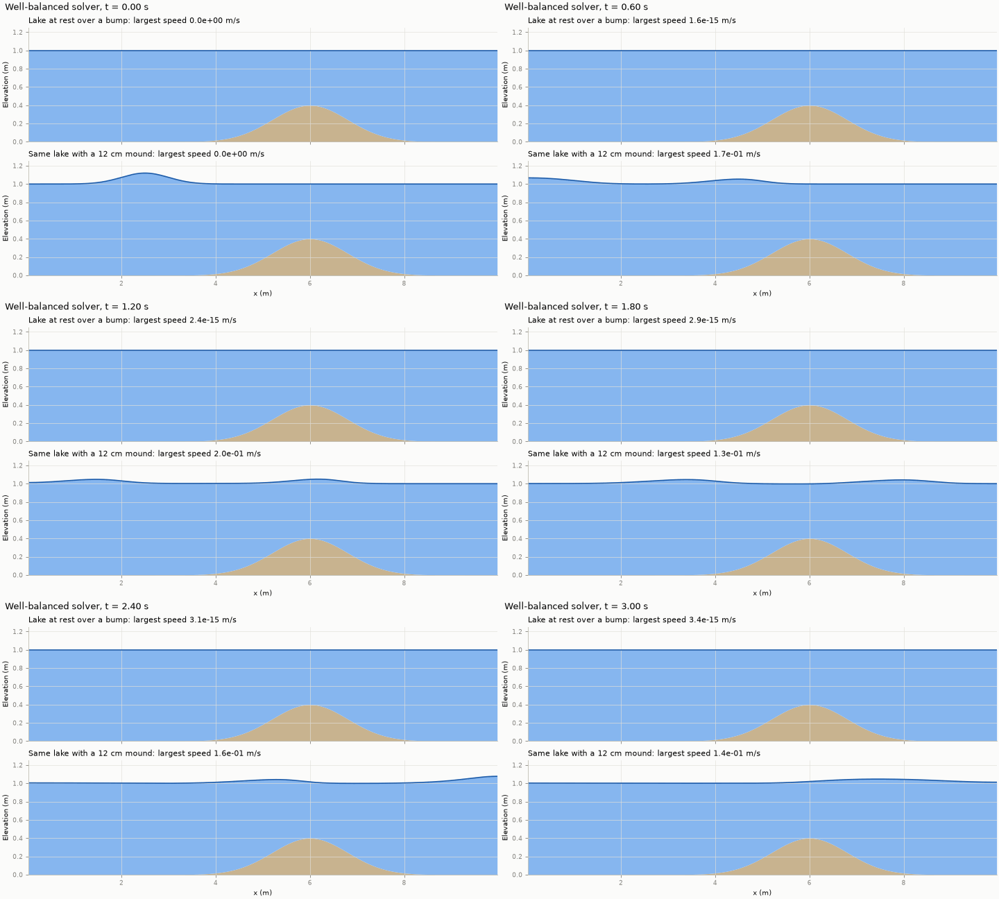
If the free surface is flat and nothing moves, the water should stay still forever, even over a bumpy bed. Set \(q_x = q_y = 0\) in Equation \(\eqref{eq-momx}\). Only the pressure and bed terms remain, and the water stays at rest only if they cancel:
\[ \begin{equation} \frac{\partial}{\partial x}\!\left(\frac12 g h^2\right) + g h\, \frac{\partial z_b}{\partial x} = g h \frac{\partial h}{\partial x} + g h \frac{\partial z_b}{\partial x} = g h\, \frac{\partial \eta}{\partial x}. \label{eq-well-balanced} \end{equation} \]
The pressure term pushes water away from deep regions, and the bed term pushes it downhill. Equation \(\eqref{eq-well-balanced}\) shows that their sum is proportional to the slope of the free surface, \(\partial \eta / \partial x\). A flat surface, \(\eta = \text{constant}\), makes it zero: the deeper water over a dip pushes outwards exactly as hard as gravity pulls water down into the dip. The same holds in \(y\).
A numerical method that keeps this balance exactly is called well-balanced. One that does not will create spurious currents over every hill. The seminar’s solver and the PINO physics loss (Chapter 4) are both well-balanced; Figure 5 shows what that means in practice.
6.2 Wet and dry: the inundation challenge
Inundation is, by definition, water moving onto dry land. At the edge of the flood, \(h \to 0\):
- Velocity \(u = q_x/h\) becomes a ratio of two vanishing numbers.
- Depth must stay non-negative, and a careless scheme can produce negative depths.
- The shoreline is a moving boundary whose location is part of the solution.
Robust wetting and drying is one of the hardest parts of practical flood modelling. To keep this seminar’s comparisons clean, all our scenarios stay fully wet. We return to what this means for the conclusions in Chapter 5.
7 Solving the equations on a computer
Except in special cases such as Figure 3, the SWE must be solved numerically. The seminar’s reference solver uses the finite-volume method, the standard approach in operational flood models.
7.1 Finite volumes
Divide the domain into \(N_x \times N_y\) rectangular cells. In each cell \((i,j)\) store the cell average \(\mathbf U_{ij}\). Integrating Equation \(\eqref{eq-conservative}\) over a cell, the divergence of the flux becomes the sum of fluxes through the four faces:
\[ \begin{equation} \frac{d\mathbf U_{ij}}{dt} = -\frac{\mathbf F_{i+\frac12,j} - \mathbf F_{i-\frac12,j}}{\Delta x} - \frac{\mathbf G_{i,j+\frac12} - \mathbf G_{i,j-\frac12}}{\Delta y} + \mathbf S_{ij}. \label{eq-fv} \end{equation} \]
Whatever leaves one cell through a face enters its neighbour. The method therefore conserves mass by construction, up to the tiny round-off errors of computer arithmetic. It also copes with shocks, because it never needs the derivative of the solution, only the fluxes between cells.
7.2 Numerical fluxes
At each face, two different states meet: \(\mathbf U_L\) from the left cell and \(\mathbf U_R\) from the right. The solver combines them with the Rusanov (local Lax–Friedrichs) flux:
\[ \begin{equation} \mathbf F_{i+\frac12} = \frac12\Big(\mathbf F(\mathbf U_L) + \mathbf F(\mathbf U_R)\Big) - \frac12\, a_{\max} \big(\mathbf U_R - \mathbf U_L\big), \label{eq-rusanov} \end{equation} \]
where \(a_{\max}\) is the fastest signal speed at the face: the flow speed plus the wave speed \(\sqrt{gh}\) of Equation \(\eqref{eq-wave}\), taking the larger of the two sides:
\[ \begin{equation} a_{\max} = \max\Big(|u_L| + \sqrt{g h_L},\ |u_R| + \sqrt{g h_R}\Big). \label{eq-signal-speed} \end{equation} \]
The first term is a simple average. The second adds numerical diffusion, proportional to the jump between the two states and the fastest local wave speed. This keeps the scheme stable, but it also smooths the solution, as the 100-cell curve in Figure 3 shows.
On a bumpy bed one more step is needed. Hydrostatic reconstruction adjusts the two face states for the difference in bed height between the cells, so that for a lake at rest the pressure and bed terms cancel exactly, as in Equation \(\eqref{eq-well-balanced}\).
7.3 Time stepping and the CFL condition
The solver advances Equation \(\eqref{eq-fv}\) in small time steps, each computed directly from the state at the previous step (an explicit scheme). For such a scheme to stay stable, a wave must not cross more than one cell per step. This limits the step to
\[ \begin{equation} \Delta t \le \mathrm{CFL}\cdot \frac{\min(\Delta x, \Delta y)}{\max\big(|\mathbf u| + \sqrt{g h}\big)}, \label{eq-cfl} \end{equation} \]
where the safety factor CFL (the Courant number, after Courant, Friedrichs and Lewy) is 0.3–0.4 in our runs. Halving the cell size therefore halves the time step too: a 2D grid that is twice as fine costs about eight times as much. This scaling is the basic reason why accurate simulations are expensive.
7.4 Accuracy and grid convergence
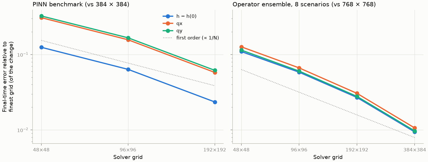
The scheme is first order: its error falls roughly in proportion to the cell size. Halve the cells and the error halves.
Throughout the seminar we measure error relative to the change. The error of a field is divided by how much that field has changed since \(t = 0\). A score of 0.1 means the error is a tenth of the change. A “prediction” that nothing changes at all scores exactly 1. This is a fair yardstick for waves, which change the water depth by only a few per cent of its total.
Figure 6 measures the solver’s error on the two problems used later: the single test problem of Chapter 2 (left, the “PINN benchmark”) and the scenarios of Chapters 3–5, described at the end of this chapter (right). On a 48 × 48 grid, the discharge error relative to the change is about 31% for the first and about 12% for the second.
This has a direct consequence for the rest of the seminar. A reference solution is only as good as its grid. The learned models work on a 48 × 48 grid, but their training data are solved on a 768 × 768 grid and then block-averaged to 48 × 48. Each coarse cell is the mean of the 16 × 16 fine cells inside it, which preserves total volume exactly. These averaged fields are the labels: the answers a model is trained to reproduce and scored against. The models therefore target the accurate solution, and the solver run directly on 48 × 48 becomes a fair “traditional” baseline at the same resolution: a standard method that any new one should beat.
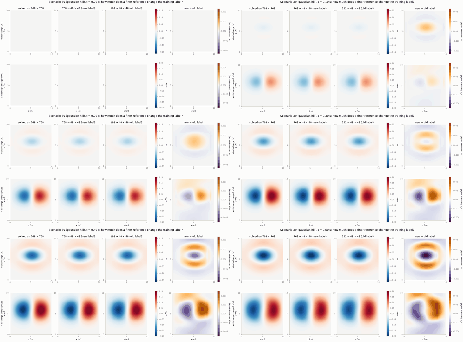
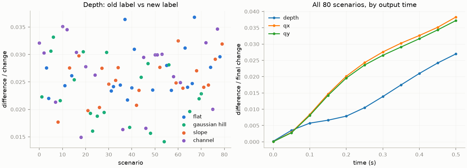
How fine is fine enough? Figure 7 compares the 768 × 768 reference with an earlier 192 × 192 one, both averaged to 48 × 48. The two sets of labels differ by about 2.5% of the change in depth and 3–3.4% in discharge (Figure 8). The difference sits on the moving wave, where the coarser solve smooths the crests and troughs, and it grows steadily with time.
How far is each from the exact solution? The 768 × 768 cells are four times smaller, so for a first-order scheme their error should be about a quarter of the 192 × 192 error. The difference between the two is then about three quarters of the 192 × 192 error. A difference of 2.5–3.4% therefore puts the 192 × 192 labels about 3.5–4.5% from the exact solution, and the 768 × 768 labels about 1%.
7.5 Verifying the solver
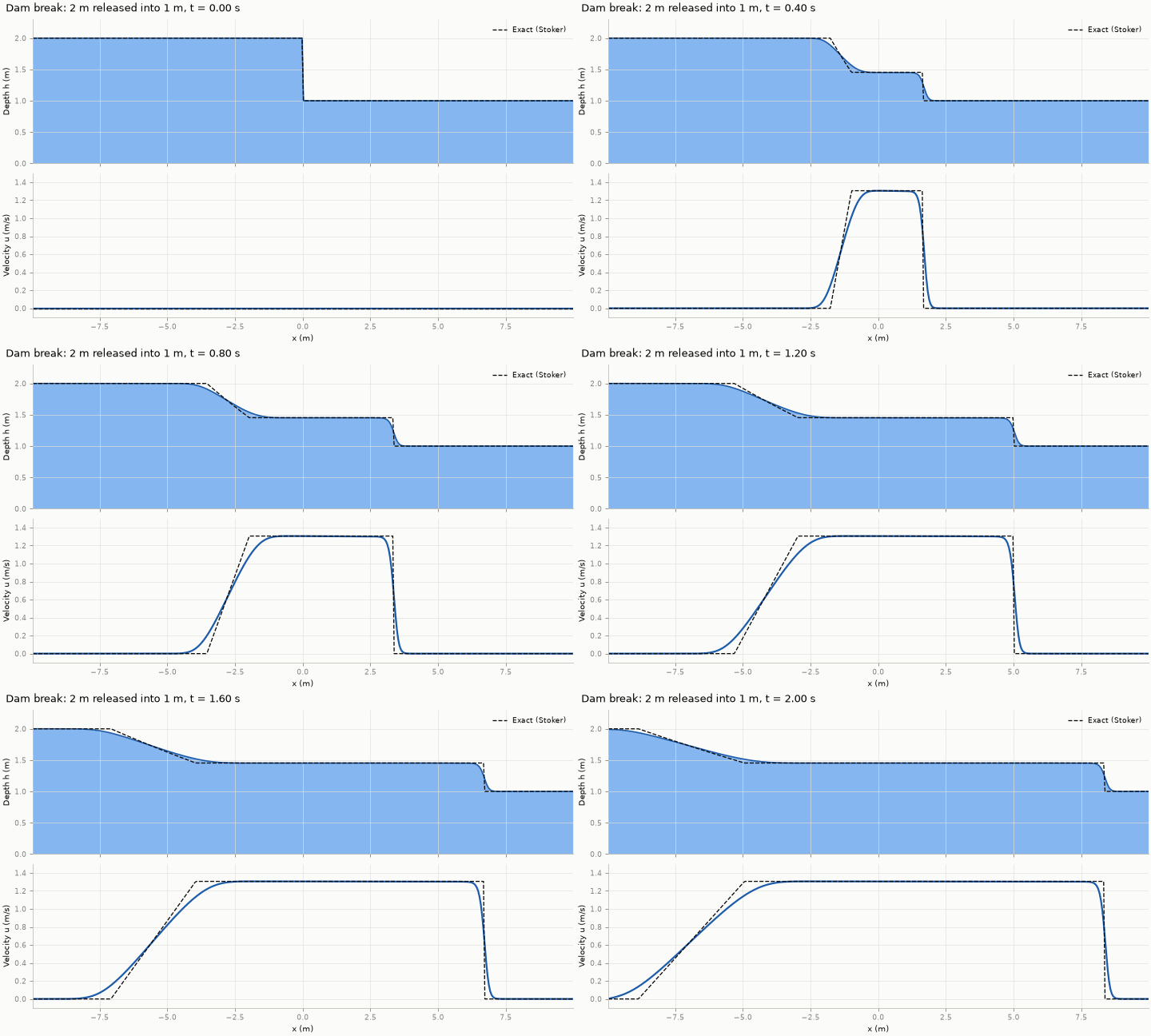
Before trusting a solver, we check it against problems whose answers we know: the lake at rest (Figure 5), the dam break (Figure 3 and Figure 4) and the radial dam break (Figure 2). Each test compares the solver with the known answer and checks that mass is conserved. Notebook 1 of the hands-on folder runs the first two.
8 The seminar’s scenario family
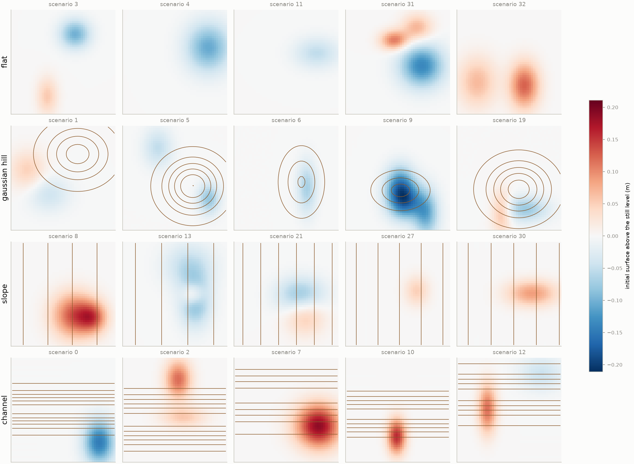
The learning chapters use one family of synthetic scenarios. Each one is a square basin, 10 m × 10 m, closed by walls, with no friction, rain or inflow. A scenario is set by three random choices: the shape of the bed, a disturbance on the water surface, and a background current. The water is then left to move under gravity alone. Everything a model is later asked to predict follows from these initial fields.
There are 80 scenarios, 20 for each of four terrain families. All random draws start from one fixed seed for the random-number generator, so the generator reproduces the same 80 scenarios on any machine.
8.1 The bed
In every family, the bed’s height scale \(A\) is drawn between 8 and 28 cm.
| Family | Bed \(z_b(x, y)\) | Other random parameters |
|---|---|---|
| Flat | \(0\) | none |
| Gaussian hill | \(A \exp\!\left[-\tfrac12\left(\tfrac{(x-x_0)^2}{\sigma_x^2} + \tfrac{(y-y_0)^2}{\sigma_y^2}\right)\right]\) | centre in the middle half of the basin; widths \(\sigma_x, \sigma_y\) of 1.0–2.2 m |
| Planar slope | \(A\, x / L\), rising towards \(+x\) | none: a gradient of 0.8–2.8% |
| Channel | \(A \left\{1 - \exp\!\left[-\tfrac12 (y-y_0)^2/\sigma^2\right]\right\}\) | a trough along \(x\); centre \(y_0\) at 3.5–6.5 m, half-width \(\sigma\) of 0.8–1.6 m |
8.2 The initial water
- Still level. The undisturbed surface lies 1.4–1.9 m above the bed’s lowest point.
- Surface disturbance. One to three Gaussian mounds or dips are added to that level: 25 scenarios have one, 30 have two and 25 have three. Each has an amplitude of ±4–16 cm, widths of 0.6–1.8 m and a centre at least 1.5 m from the walls. Mounds and dips are about equally common (83 and 77). Where two overlap, the surface can be displaced by up to about 20 cm.
- Background current. One or two smooth swirling patterns are added. Each is built from a streamfunction \(\psi \propto \sin(m\pi x/L)\,\sin(n\pi y/L)\), whose slopes give the velocity (\(u = \partial\psi/\partial y\), \(v = -\partial\psi/\partial x\)). A flow built this way neither creates nor removes water anywhere. Because \(\psi\) is zero on the walls, the flow runs along the walls and never through them. The first pattern is always a single basin-wide swirl, or gyre (\(m = n = 1\)); the second, if present, has \(m, n \in \{1, 2\}\). The top speed is between 0.5 and 22 cm/s.
Every scenario starts, and stays, fully wet: the depth stays between 1.16 and 2.01 m. Figure 9 shows the range of initial surfaces and beds, five training scenarios per family.
8.3 What happens in a run
Figure 10 follows one scenario per family through 0.5 s, the horizon of the main benchmark: the span of time the models must predict. Each mound collapses under its own weight and each dip fills in. Both send out a ring-shaped wave at 3–4 m/s, which adds its own flow to the background current on the bottom row. The current itself changes slowly. Outputs are stored every 0.05 s.
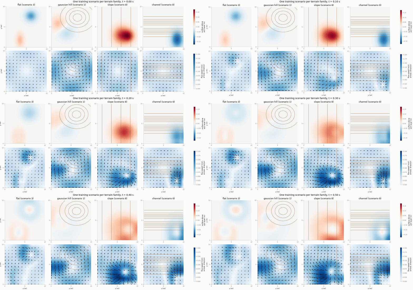
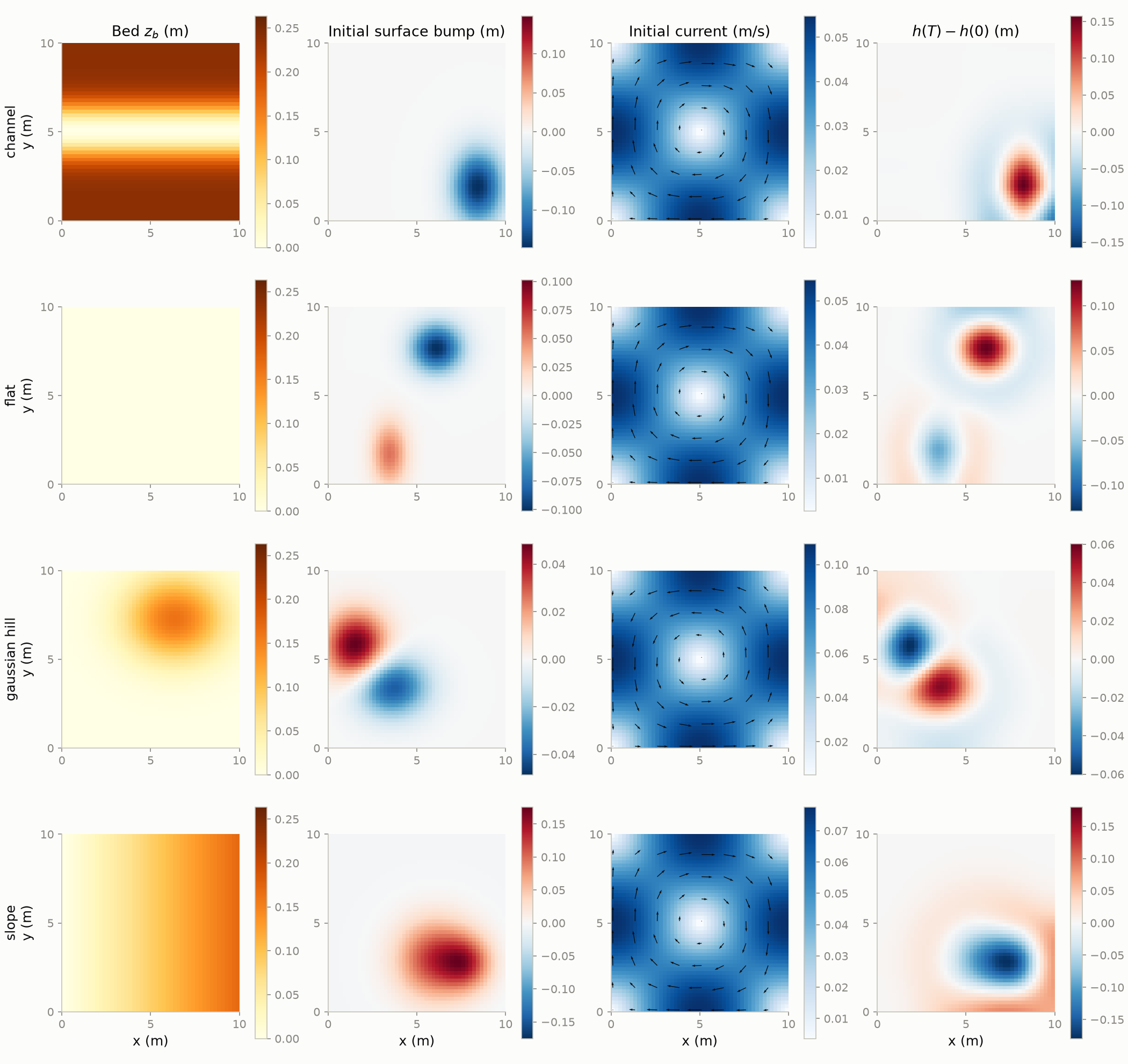
Figure 11 shows the same four scenarios as model inputs and the response the models must learn: the change in depth at the final time.
The same 80 scenarios are also run five times longer, to 2.5 s, with 51 stored times. This is long enough for the rings to reach the walls after about 0.5–1 s, reflect and cross one another. By the end the surface is a pattern of overlapping waves rather than isolated rings, and the bed visibly steers it. This longer run is a much harder prediction task.
The animations below follow one 2.5 s scenario per family, one per tab. The two left panels are the view from above, as in Figure 10: the surface, and the current with arrows for its direction, over the bed contours. The right panels cut the basin along the dashed line, as in Figure 5. The upper one is a side view at true scale, showing the bed and the water above it. The lower one is the surface along the same line on a stretched scale, so that waves a few centimetres high can be read.
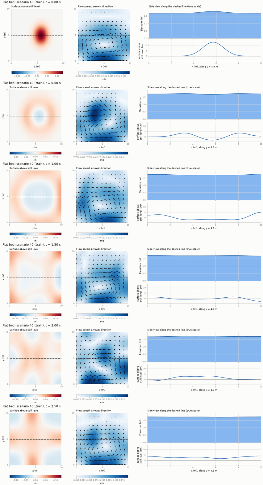
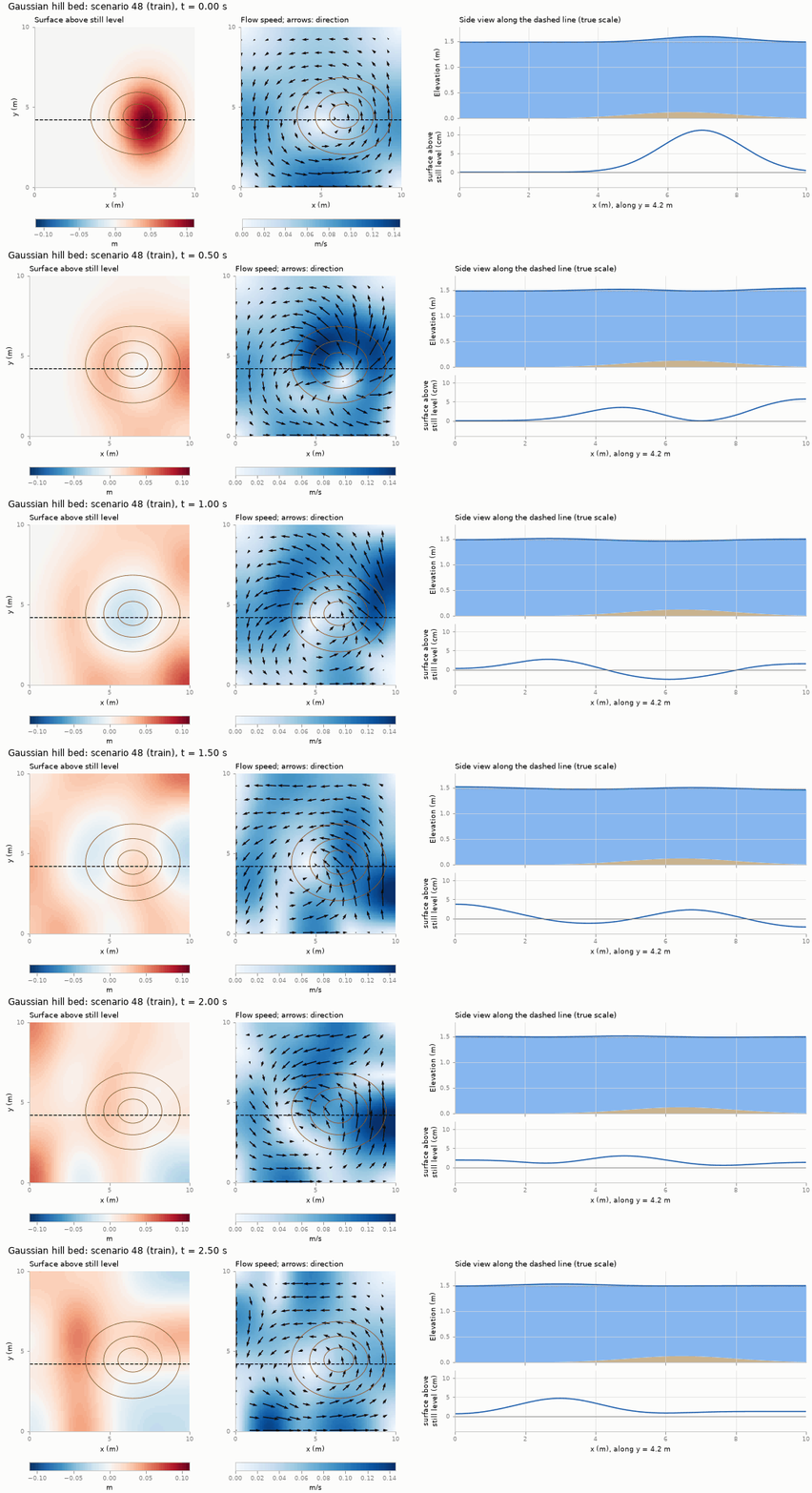
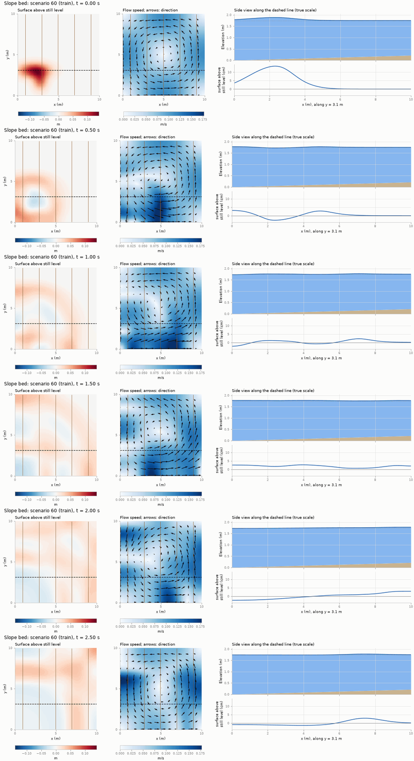
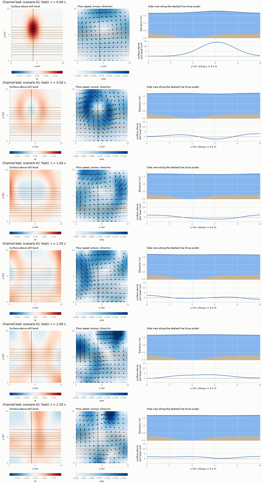
These runs were solved again on a 384 × 384 grid for the animations, so that the side views are sharp; the stored data are the 48 × 48 averages of the 768 × 768 runs.
The dataset’s slope is gentle: the depth changes by at most 28 cm in about 1.6 m of water. A tsunami meets something much stronger. In the open ocean it is a long, low wave, often less than a metre high in water several kilometres deep. Near the coast the water becomes shallow, and the wave slows down, shortens and grows. Figure 16 shows this on a small scale with the seminar’s solver. It is not one of the dataset’s scenarios.
In linear theory, a long wave that moves into slowly shallowing water keeps its energy flux, and its height \(a\) grows as the depth falls, following Green’s law: \[ a \propto h^{-1/4}. \] Going from 1 m of water to 5 cm, this predicts a wave about 2.1 times higher. The wave’s crest also travels faster than its trough, because the crest stands in deeper water; in shallow water this steepens the front until it becomes a bore, which loses energy as it runs on.
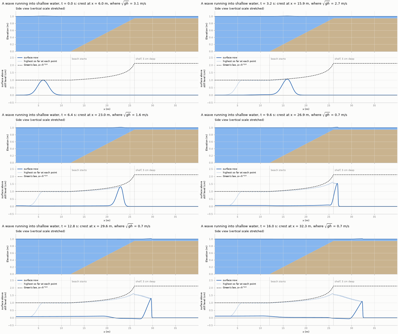
Table 3 puts numbers on this regime. It helps to keep these in mind when interpreting results.
| Quantity | Value | Consequence |
|---|---|---|
| Wave speed \(c=\sqrt{gh}\) | 3.3–4.3 m/s | Fast compared with the currents |
| Distance travelled in 0.5 s | about 2 m | A ring has not yet reached most walls |
| Time to cross the basin | about 2.5 s | Wall reflections mostly lie beyond the horizon |
| Amplitude ratio \(\varepsilon\) | about 0.02–0.1 | Weakly nonlinear |
| Froude number | below about 0.1 | Subcritical: no bores or shocks |
The scenarios are divided into three groups, 14/3/3 per terrain family:
- 56 training scenarios, which the models learn from;
- 12 validation scenarios, used to choose settings such as the network size or loss weights;
- 12 test scenarios, used only for the final scores.
Each scenario belongs to exactly one group, as a whole. No test scenario is seen during training or used to choose settings, so the test scores measure performance on genuinely new scenarios.
8.4 The stored datasets
Each dataset stores, for every scenario, the inputs (bed, initial depth and initial discharges \(q_x, q_y\)) and the targets (\(h, q_x, q_y\) at every stored time). The same scenarios are stored in several versions:
| Dataset | Horizon (stored times) | Grid (solved on) | Used for |
|---|---|---|---|
| Main benchmark | 0.5 s (11) | 48 × 48 (768 × 768) | Chapters 3–5 |
| Main benchmark, finer average | 0.5 s (11) | 96 × 96 (768 × 768) | testing a model on a finer grid than it was trained on, Chapter 3 |
| Longer horizon | 2.5 s (51) | 48 × 48 (768 × 768) | the longer-horizon test |
| Earlier reference | 0.5 s (11) | 48 × 48 (192 × 192) | the scarce-data and physics-weight studies, Chapter 4 |
| Unlabelled | 0.5 s | 48 × 48 | 240 further scenarios from another seed. Only their initial fields are used, not their solutions (labels), Chapter 4 |
| Fine fields | 0.5 s (11) and 2.5 s (every 5th) | 768 × 768 | full-resolution solutions of the validation and test scenarios (test only at 2.5 s), to check in future whether models can recover detail finer than their grid |
Generating the main benchmark is the most expensive step of the seminar. Each scenario is solved once on 768 × 768 cells, which takes several hours for all 80, even with 8 parallel workers. The fine solution is averaged to 96 × 96, for a resolution test in Chapter 3, and again to the 48 × 48 training grid. The longer-horizon dataset takes about five times as long. For a few chosen scenarios the full-resolution fields are kept as well. The hands-on folder contains the finished 48 × 48 dataset.
The generator records the seed, numerical settings, scenario parameters, split and mass diagnostics in a manifest stored with the data. These are teaching data, not field observations or a validated flood model.
- The shallow-water equations describe depth-averaged flow when water is much shallower than the flow is wide. They conserve mass, Equation \(\eqref{eq-mass}\), and momentum, Equations \(\eqref{eq-momx}\)–\(\eqref{eq-momy}\), written compactly as Equation \(\eqref{eq-conservative}\).
- Their key behaviour is wave propagation at speed \(c=\sqrt{gh}\). Large waves steepen into bores, which are mathematical shocks.
- A unique solution needs initial conditions, the bed and boundary conditions. Good schemes are well-balanced: they keep a lake at rest exactly at rest.
- Wet/dry fronts are the defining difficulty of inundation. Our benchmark avoids them deliberately.
- Finite-volume solvers conserve mass and capture shocks. First-order schemes add numerical diffusion, so accuracy needs fine grids, and cost grows about eightfold per halving of the cell size.
- The seminar’s data are fully wet basins solved on a fine grid and averaged to 48 × 48, over 0.5 s, and over 2.5 s for a final test.
- Why does the equation set use \(q_x = hu\) rather than \(u\)?
- A tsunami crosses 4 km deep ocean, then 10 m deep shelf water. How do its speed and its height change?
- Why must a scheme be well-balanced to simulate a lake at rest over hills?
- A grid of 48 × 48 cells takes 0.03 s per scenario. Roughly how long should 192 × 192 take? (Measured: 1.2 s.)
- Looking at Table 3, which physical processes can this benchmark not test?