flowchart LR
  P["points (x, y, t)"] --> N["network U_θ"]
  N --> AD["autodiff: ∂U/∂t, ∂F/∂x, ∂G/∂y"]
  AD --> R["PDE residual R"]
  N --> IC["initial-condition mismatch"]
  N --> BC["wall mismatch"]
  R --> L["loss L(θ)"]
  IC --> L
  BC --> L
  L -->|"gradient ∇θ L"| N
Physics-informed neural networks
Teaching a network one solution of a PDE
Learning objectives
By the end of this chapter you should be able to:
- Describe a neural network as a flexible, differentiable function, and explain how it is trained.
- Explain how automatic differentiation computes the derivatives a PDE needs.
- Build a PINN loss from PDE residuals, initial conditions and boundary conditions.
- Explain why nondimensionalisation, hard constraints and input scaling matter for training.
- Judge PINN accuracy with appropriate metrics and an appropriate reference.
- Explain why a PINN, as used here, is not a fast replacement for a solver.
1 The central idea
A classical solver represents the solution as numbers on a grid. A physics-informed neural network (PINN) represents it as a function: a neural network \(\mathbf U_\theta(x, y, t)\) that takes a point in space and time and returns the water state there. Training adjusts the network’s parameters \(\theta\) until the function satisfies the shallow-water equations, the initial condition and the boundary conditions. No simulation data are needed, although they can be added.
2 A short primer on neural networks
2.1 A network is a function with adjustable parameters
The simplest network, a multilayer perceptron (MLP), alternates two operations. An affine map multiplies its input by a weight matrix and adds a bias vector. A nonlinear activation \(\sigma\), such as \(\tanh\), is then applied to each entry:
\[ \begin{equation} \mathbf z_1 = \sigma(W_1 \mathbf x + \mathbf b_1),\quad \mathbf z_2 = \sigma(W_2 \mathbf z_1 + \mathbf b_2),\quad \dots,\quad \mathbf U_\theta(\mathbf x) = W_L \mathbf z_{L-1} + \mathbf b_L. \label{eq-mlp} \end{equation} \]
The parameters \(\theta = \{W_k, \mathbf b_k\}\) are the numbers we tune. Our PINNs use five hidden layers (the layers between input and output) of 64 units each, about 17,000 parameters. With enough units an MLP can approximate any smooth function. This is the universal approximation property, and it says nothing about how easy the right parameters are to find.
2.2 Training is minimising a loss
We define a loss \(\mathcal L(\theta)\) that is small when the network does what we want, and minimise it by gradient descent:
\[ \begin{equation} \theta \leftarrow \theta - \alpha\, \nabla_\theta \mathcal L(\theta), \label{eq-gd} \end{equation} \]
with a small learning rate \(\alpha\). We use Adam, a variant that adapts the step for each parameter. Each update is an iteration; an epoch is one pass over the training points.
2.3 Automatic differentiation
A PDE involves derivatives such as \(\partial h/\partial t\). Because the network is a composition of simple differentiable operations, the chain rule gives these derivatives exactly, not by finite differences. Automatic differentiation (autodiff) applies the chain rule mechanically, and it is the same machinery that computes \(\nabla_\theta \mathcal L\) for training. In PyTorch one call, torch.autograd.grad, returns \(\partial \mathbf U_\theta / \partial (x, y, t)\) at any set of points.
3 The PINN loss
Pick random collocation points \((x_k, y_k, t_k)\) inside the space–time domain. At each one, evaluate the network and its derivatives, and substitute them into the PDE written as “left-hand side minus right-hand side”. What is left over, the amount by which the equation fails at that point, is the residual. For the conservative SWE of Chapter 1 it is
\[ \begin{equation} \mathbf R_\theta = \frac{\partial \mathbf U_\theta}{\partial t} + \frac{\partial \mathbf F(\mathbf U_\theta)}{\partial x} + \frac{\partial \mathbf G(\mathbf U_\theta)}{\partial y} - \mathbf S(\mathbf U_\theta, z_b). \label{eq-residual} \end{equation} \]
An exact solution has \(\mathbf R = 0\) everywhere. The loss adds up the squared residual and the mismatch with the initial and boundary conditions:
\[ \begin{equation} \mathcal L(\theta) = \underbrace{\frac{1}{N_r}\sum_{k} \big|\mathbf R_\theta(x_k,y_k,t_k)\big|^2}_{\mathcal L_{PDE}} + w_I \underbrace{\frac{1}{N_I}\sum_{k} \big|\mathbf U_\theta(x_k,y_k,0) - \mathbf U_0(x_k,y_k)\big|^2}_{\mathcal L_{IC}} + w_B\, \mathcal L_{BC}. \label{eq-pinn-loss} \end{equation} \]
The weights \(w_I\) and \(w_B\) balance the terms. Choosing them is a known difficulty of PINNs. Too small, and the network finds a smooth function that satisfies the PDE but not the problem. Too large, and it fits the conditions while ignoring the physics.
4 Step 1: linear waves with a known answer
We first check the machinery on a problem with an exact solution: the linearised equations of Chapter 1, over constant depth \(H\). With free-surface displacement \(\eta\):
\[ \begin{equation} \eta_t + H(u_x + v_y) = 0,\qquad u_t + g\eta_x = 0,\qquad v_t + g\eta_y = 0. \label{eq-linear-2d} \end{equation} \]
On a periodic square of side \(L\), one where a wave leaving through one side re-enters through the opposite side, a plane wave travelling diagonally solves them exactly:
\[ \begin{equation} \eta = A \sin\!\left(2\pi\left(\frac{x}{L} + \frac{y}{L} - \sqrt{2}\,\frac{c t}{L}\right)\right),\qquad u = v = \frac{c}{\sqrt 2\, H}\,\eta,\qquad c=\sqrt{gH}. \label{eq-plane-wave} \end{equation} \]
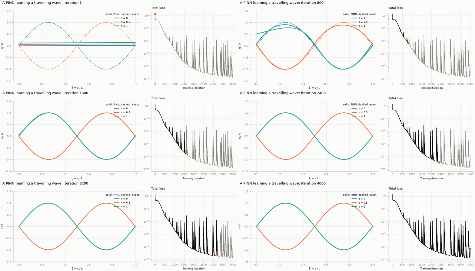
Figure 1 shows the 1D version of this problem, a wave travelling in \(x\) only, being learned. Time is shown as \(\tau\), the time in units of how long the wave takes to cross the square (defined in Equation \(\eqref{eq-scales}\) below). At first the network outputs almost nothing. It soon matches the initial wave at \(\tau = 0\), which is the easiest condition to fit, and only later gets the wave right at later times, where it depends on the PDE residual alone.
4.1 Nondimensionalisation
Physical variables have very different sizes: \(x\) in metres, \(\eta\) in centimetres, \(t\) in fractions of a second. Networks train best when inputs and outputs are of order one. We therefore rescale by the natural scales of the problem:
\[ \begin{equation} \xi = \frac{x}{L},\quad \zeta = \frac{y}{L},\quad \tau = \frac{c t}{L},\quad \hat\eta = \frac{\eta}{A},\quad \hat u = \frac{H u}{c A},\quad \hat v = \frac{H v}{c A}, \label{eq-scales} \end{equation} \]
which turns Equation \(\eqref{eq-linear-2d}\) into a parameter-free system:
\[ \begin{equation} \hat\eta_\tau + \hat u_\xi + \hat v_\zeta = 0,\qquad \hat u_\tau + \hat\eta_\xi = 0,\qquad \hat v_\tau + \hat\eta_\zeta = 0. \label{eq-linear-nd} \end{equation} \]
The network maps \((\xi, \zeta, \tau) \mapsto (\hat\eta, \hat u, \hat v)\). Its loss contains the three residuals of Equation \(\eqref{eq-linear-nd}\), the initial condition, and periodicity in both directions.
Notebook 2 of the hands-on folder trains the one-dimensional warm-up in about a minute. Compare runs by their solution errors, not their final training losses: a loss mixes several terms whose balance depends on the weights.
5 Step 2: the nonlinear equations over a bump
The real test uses the full nonlinear SWE, Equation \(\eqref{eq-residual}\), over a smooth Gaussian hill, in a 4 m walled basin about 1 m deep. Initially the water is at rest, with a 6 cm mound on the surface away from the hill. As in Equation \(\eqref{eq-scales}\), lengths are scaled by \(L\), depths by the still depth \(H\), discharges by \(H\sqrt{gH}\) and time by \(L/\sqrt{gH}\). The dimensionless equations then have \(g = 1\).
There is no exact solution, so the PINN is compared with the finite-volume solver of Chapter 1.
5.1 Measuring the right thing, against the right reference
The first nonlinear PINN appeared to work: total-depth error 0.6%. Two measurement problems sat behind that number.
- Total depth hides the wave. The water column is about 1 m and the wave about 6 cm, so even a flat, motionless prediction scores a small relative error on \(h\). The meaningful quantity is the change \(h(t) - h(0)\). On that scale the early PINN was 46% wrong, as wrong in depth as in discharge.
- The reference was too coarse. On 48 × 48 cells the first-order solver is itself about 31% wrong in discharge (Chapter 1, grid convergence figure). A PINN approximates the continuous equations, so it must be judged against a much finer solution. All errors below are measured against a 384 × 384 solve, averaged to 48 × 48.
This is why, as introduced in Chapter 1, errors are reported relative to the size of the change:
\[ \begin{equation} e_{q} = \frac{\big\| q_{\text{pred}} - q_{\text{ref}} \big\|_2}{\big\| q_{\text{ref}} - q_{\text{ref}}(t{=}0) \big\|_2}, \label{eq-change-error} \end{equation} \]
where \(\|\cdot\|_2\) is the square root of the sum of squares over all grid cells and all output times after \(t=0\). A prediction of “nothing happens” scores exactly 1, and a perfect prediction scores 0.
5.2 Hard constraints: build the conditions into the network
The initial- and boundary-condition terms in Equation \(\eqref{eq-pinn-loss}\) are penalties: they discourage violations but do not prevent them, and they compete with the PDE term. A better option, where possible, is to construct the network output so that a condition holds exactly for every \(\theta\). Let \(\mathbf N_\theta\) be the raw MLP output. The improved PINN uses
\[ \begin{equation} h = h_0(\xi,\zeta)\, e^{\tau N^{(h)}_\theta},\qquad q_x = 4\xi(1-\xi)\, \tau N^{(x)}_\theta,\qquad q_y = 4\zeta(1-\zeta)\, \tau N^{(y)}_\theta. \label{eq-hard} \end{equation} \]
- At \(\tau = 0\) the exponential is 1, so \(h = h_0\), and both discharges vanish. The initial condition holds exactly.
- The factor \(4\xi(1-\xi)\) is zero on the walls \(\xi = 0\) and \(\xi = 1\), so the normal discharge vanishes there exactly. The factor in \(\zeta\) does the same for the other pair of walls.
- The exponential keeps \(h\) positive.
Only the PDE loss is then left to balance.
Two further changes help the optimiser:
- Input centring maps each input to \([-1, 1]\), where \(\tanh\) layers are most sensitive.
- Collocation resampling draws fresh random points every epoch, so the network cannot satisfy the PDE only at a fixed set of points.
5.3 Results
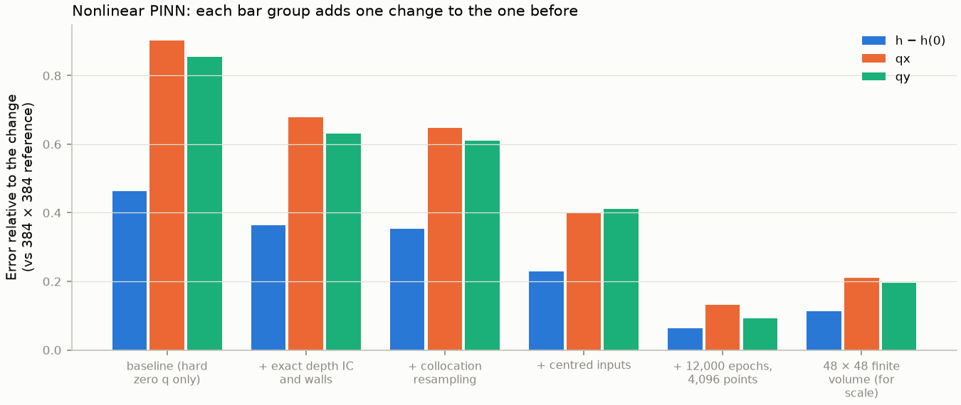
Figure 2 adds one change at a time, and Table 1 gives the numbers.
| Experiment (cumulative) | seeds | total depth | depth anomaly | qx | qy | fresh-point PDE loss |
|---|---|---|---|---|---|---|
| baseline (hard zero q only) | 1 | 0.006 | 0.463 | 0.903 | 0.855 | 1.7e-04 |
| + exact depth IC and walls | 1 | 0.005 | 0.364 | 0.679 | 0.631 | 1.2e-03 |
| + collocation resampling | 1 | 0.004 | 0.352 | 0.648 | 0.610 | 1.1e-03 |
| + centred inputs | 1 | 0.003 | 0.228 | 0.401 | 0.412 | 4.7e-04 |
| + 12,000 epochs, 4,096 points | 3 | 0.001 ± 0.000 | 0.064 ± 0.003 | 0.133 ± 0.010 | 0.092 ± 0.003 | 5.4e-05 |
| 48 x 48 finite-volume solution, for scale | - | 0.001 | 0.113 | 0.210 | 0.196 | - |
What the table teaches:
- Exact constraints help even though the PDE loss rises. Training losses from different formulations are not comparable; only solution errors are.
- Small engineering choices matter. Input centring alone cut the discharge error from about 0.65 to 0.40.
- Training budget matters most. The final configuration (12,000 epochs, 4,096 points, three seeds) gets within 6% in depth change and 9–13% in discharge.
- Seeds. Training is random: the starting weights and the collocation points are drawn from a random-number generator, fixed by a seed. Repeating a run with different seeds shows how much a result owes to luck. Only the last row has three seeds. The other rows are single runs, so small differences between neighbouring rows should not be over-read.
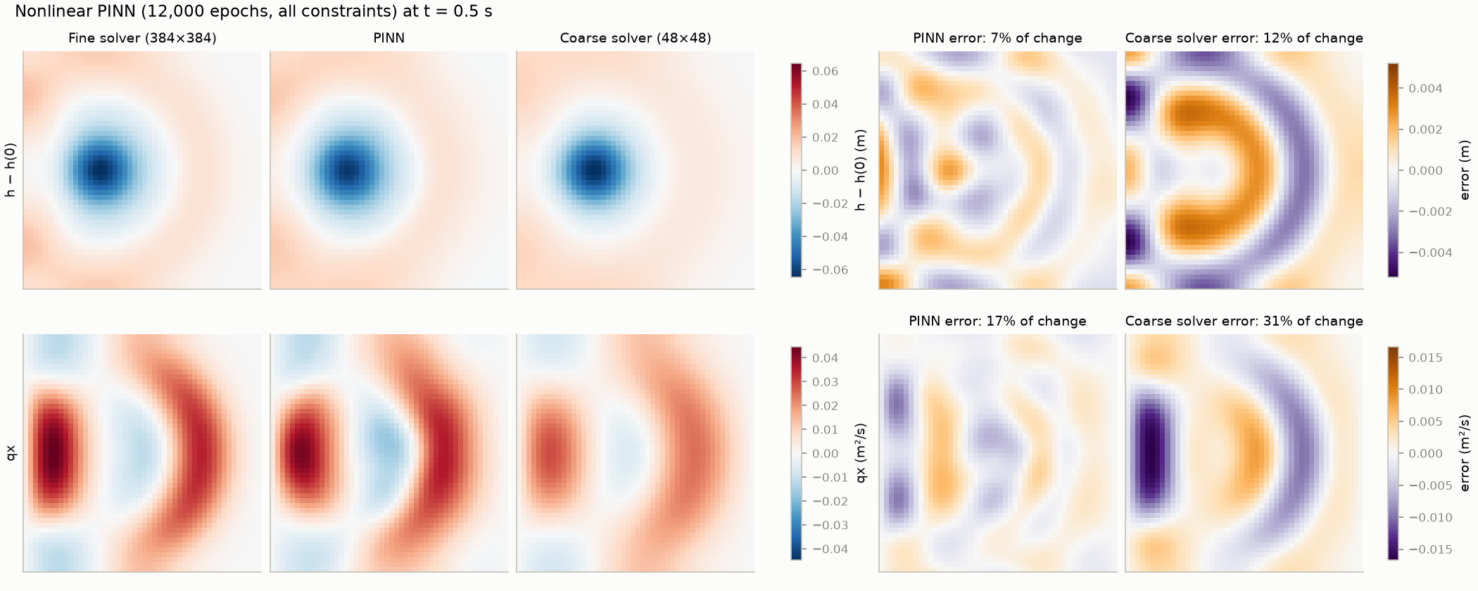
Figure 3 shows the PINN beating the 48 × 48 solver at its own resolution. The PINN has no grid, so it does not suffer numerical diffusion; its error comes from imperfect optimisation instead.
The best run takes 30–60 minutes on a multi-core CPU.
5.4 Is a PINN a fast solver?
No, not in this form. The PINN took tens of minutes to learn one scenario. A finer finite-volume solve of the same scenario takes about a second and is more accurate. Change the initial mound or the hill, and the PINN must be retrained from scratch.
PINNs are attractive where solvers struggle: inverse problems (inferring an unknown parameter, such as bed friction, from sparse observations), irregular data, or geometries that are hard to cover with a grid. For fast prediction across many scenarios we need a model that learns the mapping from scenario to solution. That is the subject of Chapter 3.
Summary
- A PINN is a neural network \(\mathbf U_\theta(x,y,t)\) trained so that the PDE residual Equation \(\eqref{eq-residual}\), the initial condition and the boundary conditions are small. Automatic differentiation supplies exact derivatives.
- Nondimensionalisation Equation \(\eqref{eq-scales}\) and centred inputs keep the optimisation well-scaled.
- Hard constraints Equation \(\eqref{eq-hard}\) make initial and wall conditions exact, leaving only the PDE to learn.
- Evaluate the change in the solution, Equation \(\eqref{eq-change-error}\), against a reference that is more accurate than the model.
- The best PINN beats the 48 × 48 solver, but costs far more than a fine solve and must be retrained for every scenario.
Check your understanding
- Why does a PINN need no simulation data, at least in principle?
- In Equation \(\eqref{eq-hard}\), what would go wrong if \(h\) were written as \(h_0 + \tau N^{(h)}_\theta\)?
- A colleague reports that their PINN’s total loss fell by a factor of 100. What else would you ask before believing it is accurate?
- Why did the 48 × 48 solver make a poor reference for the PINN, but a fair baseline for the operators in Chapter 3?