Neural operator learning
Learning the map from a scenario to its solution
By the end of this chapter you should be able to:
- Distinguish learning one solution (a PINN) from learning a solution operator.
- Describe the DeepONet and Fourier Neural Operator (FNO) architectures, and the role of the Fourier transform in an FNO.
- Explain why non-periodic walls need special care in an FNO.
- Explain three design choices that made the seminar’s FNO work: predicting the change, symmetry augmentation, and refined training data.
- Set up a fair evaluation, with scenario-level splits, baselines and metrics relative to the change.
- Read the comparison between the FNO and a traditional solver, including where each one wins.
1 From one solution to a solution operator
The PINN of Chapter 2 learned one function, \(\mathbf U(x,y,t)\), for one fixed bed and initial state. Change the initial mound and the PINN is useless.
The finite-volume solver of Chapter 1 is different in kind. It takes any bed and initial state, and returns the corresponding solution. Mathematically, it approximates the solution operator
\[ \begin{equation} \mathcal G : \underbrace{(z_b,\ \mathbf U_0)}_{\text{input functions}} \longmapsto \underbrace{\mathbf U(\cdot,\cdot,t)}_{\text{output functions}}, \label{eq-operator} \end{equation} \]
a map from functions to functions. Operator learning trains a network \(\mathcal G_\theta \approx \mathcal G\) on many example pairs (input → solution), produced by the solver. After training, a new scenario costs one network evaluation instead of one simulation.
A useful analogy:
- A PINN is like memorising the answer to one exam question.
- An operator is like learning to answer any question of that type.
The second is far more useful, but it needs many worked examples.
1.1 What the seminar’s operator maps
On the 48 × 48 grid, the input is six fields: the bed, the three fields of the initial state, and the \(x\) and \(y\) coordinates of each cell. The output is the state at ten times:
\[ \begin{equation} \mathcal G_\theta:\ \big(z_b,\ h_0,\ q_{x,0},\ q_{y,0},\ x,\ y\big) \longmapsto \big(h, q_x, q_y\big)(t_k),\qquad t_k = 0.05\,k\ \text{s},\ k = 1,\dots,10. \label{eq-our-operator} \end{equation} \]
All ten output times come from one forward pass, a single evaluation of the network. The model never steps forward in time, so errors cannot accumulate from step to step.
2 Two architectures
2.1 DeepONet
DeepONet (Lu et al. 2021) rests on a theorem: any continuous operator can be approximated as a sum of products. One network, the branch, reads samples of the input function \(a\) and outputs \(p\) coefficients. A second network, the trunk, reads an output coordinate \(\mathbf y = (x, y, t)\) and outputs \(p\) values, one for each of \(p\) learned patterns. The prediction is the sum of their products:
\[ \begin{equation} \mathcal G_\theta(a)(\mathbf y) = \sum_{k=1}^{p} \underbrace{b_k(a)}_{\text{branch}}\ \underbrace{\phi_k(\mathbf y)}_{\text{trunk}}. \label{eq-deeponet} \end{equation} \]
You can read this as a learned version of the classical trick of writing a solution as a sum of simple patterns: the trunk learns the patterns, and the branch learns how much of each pattern a given scenario needs. The seminar introduces DeepONet conceptually and implements the FNO.
2.2 The Fourier Neural Operator
The FNO (Li et al. 2021) treats the input as an image-like stack of fields and transforms it through a sequence of layers.
- A lift \(P\) maps the 6 input fields at each cell to a wider representation \(v_0\), with 32 fields. As with the red, green and blue layers of a colour image, each field is called a channel.
- Four Fourier layers update this representation (Equation \(\eqref{eq-fourier-layer}\)).
- A projection \(Q\) maps back to the 30 output channels: 3 variables at 10 times.
Each Fourier layer does
\[ \begin{equation} v_{\ell+1}(\mathbf x) = \sigma\Big( W_\ell\, v_\ell(\mathbf x) + \mathcal F^{-1}\big[ R_\ell(\mathbf k) \cdot \mathcal F[v_\ell](\mathbf k) \big](\mathbf x) \Big), \label{eq-fourier-layer} \end{equation} \]
where:
- \(\mathcal F\) is the 2D Fourier transform, which writes the field as a sum of sine-like waves, or modes. Each mode has a wavenumber \(\mathbf k\): how many wavelengths fit across the domain in \(x\) and \(y\). Low wavenumbers are broad, smooth patterns; high ones are fine detail.
- \(R_\ell(\mathbf k)\) is a learned matrix of complex numbers for each kept wavenumber. Only the lowest 12 modes in each direction are kept; the rest are set to zero.
- \(W_\ell\) is a linear map applied to each cell separately, which recovers local detail.
- \(\sigma\) is the GELU activation, a smooth nonlinear function that plays the role \(\tanh\) played in Chapter 2.
Why Fourier? Multiplying by \(R(\mathbf k)\) in Fourier space is equivalent to a convolution in physical space: each output cell becomes a weighted sum of all input cells, with weights that depend on the distance between them. One layer can therefore move information across the whole basin, as a wave does. Keeping only low modes builds in a preference for smooth fields, which suits smooth flows. Because \(R\) is defined per physical wavenumber, not per grid cell, the same trained weights can be applied on a finer grid (Section 5.5).
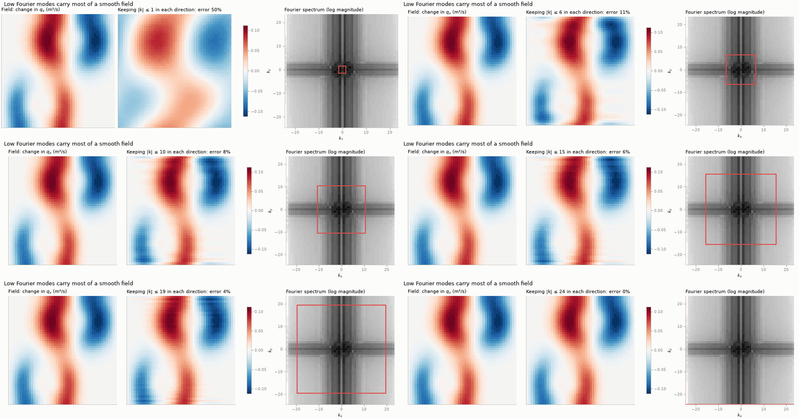
Figure 1 shows what keeping only low modes does to a typical field from our dataset. About six modes in each direction already capture the field to within about 10%. The FNO keeps twelve.
2.3 Fourier layers and walls
The discrete Fourier transform treats a field as periodic: the right edge continues into the left edge. Our basin has walls, not periodic boundaries, so an FNO applied directly would let a wave leaving the right wall “reappear” at the left one.
The standard remedy, used here, is to zero-pad the domain by 12.5% on every side before the Fourier layers and crop afterwards. This keeps the periodic wrap-around away from the physical domain. As Section 5.5 shows, this sounded necessary but did not measurably help on this benchmark.
3 Three design choices that matter
3.1 1. Predict the change, not the state
The network does not output \(\mathbf U(t_k)\) directly. It outputs a correction to the initial state that grows with time:
\[ \begin{equation} \mathcal G_\theta(\cdot)(t_k) = \mathbf U_0 + \frac{t_k}{T}\, \mathbf s \odot \mathbf N_\theta(\cdot)(t_k), \label{eq-change-param} \end{equation} \]
where:
- \(\mathbf N_\theta\) is the FNO output;
- \(T = 0.5\) s is the horizon;
- \(\mathbf s\) is the typical size of the change of each variable over the training set;
- \(\odot\) multiplies channel by channel.
Two consequences follow. At \(t=0\) the prediction is exactly the initial state. And a network that outputs zero reproduces persistence, the “nothing happens” forecast, so the network only has to learn the departure from it. This is the operator-learning counterpart of the PINN’s hard constraints in Chapter 2.
3.2 2. Symmetry augmentation
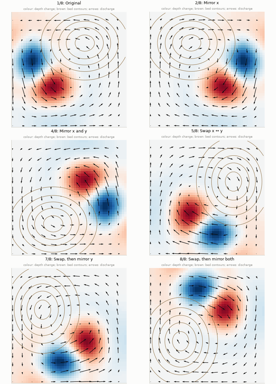
A square walled basin looks the same after mirroring left–right or top–bottom, or swapping \(x\) and \(y\): eight transformations in all. The shallow-water equations are unchanged by them, provided discharge is transformed as a vector. For example, mirroring in \(x\) maps
\[ \begin{equation} \big(z_b, h, q_x, q_y\big)(x, y) \;\mapsto\; \big(z_b, h, -q_x, q_y\big)(L - x,\, y). \label{eq-mirror} \end{equation} \]
If a scenario is a valid solution, so are its seven transformed copies. Training on randomly transformed samples therefore gives the network 8× more distinct examples at no simulation cost. The solver obeys these symmetries exactly, so every transformed copy is a genuine solution, not an approximation.
3.3 3. Train on accurate data
As Chapter 1 showed, a 48 × 48 first-order solve is about 12% off for these scenarios. The training data are therefore solved on 768 × 768 cells and block-averaged to 48 × 48. On that grid the reference itself is about 1% off; an earlier 192 × 192 reference was about 3.5–4.5% off, and some of the experiments below were run with it (they are marked). The operator learns the accurate solution at coarse resolution, which is precisely what the coarse solver cannot provide.
4 Training and evaluation
Four rules keep the evaluation fair.
- Split by scenario. The 56 training, 12 validation and 12 test scenarios are whole, independent simulations. Splitting snapshots of the same simulation between training and test would leak the answer and give misleadingly good results.
- Normalise with training data only. Each input field is rescaled to have mean 0 and standard deviation 1, which helps training. The means and standard deviations, and the change scales \(\mathbf s\), come from the training scenarios only, and they are stored with the trained weights (the checkpoint).
- Loss. For each scenario and variable, the loss is the error relative to the size of the true change, as defined in Chapter 2, averaged over scenarios. Every scenario then counts equally, whether its waves are large or small.
- Selection. The optimiser is AdamW, the Adam method of Chapter 2 with a mild penalty on large weights. Its learning rate first rises, then falls (a one-cycle schedule), over 1,000 epochs. The weights from the epoch with the lowest validation error are kept. Test scenarios are used only for the final report. Training the FNO this way takes about 25 minutes on a laptop CPU.
Baselines give the numbers meaning:
- Persistence predicts that nothing changes. By construction it scores 1 on our metric.
- The 48 × 48 solver, run from the same block-averaged initial state, is the “traditional” method at equal resolution.
5 Results
5.1 Accuracy on unseen scenarios
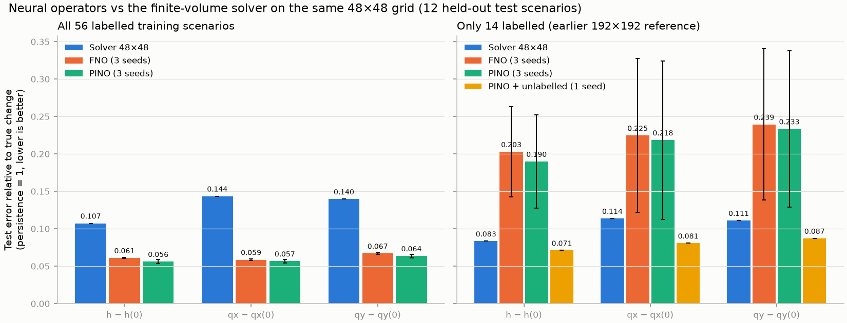
The results also show the PINO: the same network, trained with an extra term that rewards satisfying the equations. Chapter 4 explains it; for now, read it as a second operator.
| model | labelled | seeds | depth anomaly err | qx change err | qy change err | depth RMSE (m) | qx RMSE (m²/s) | qy RMSE (m²/s) | mass err | PDE residual | wall normal q (m²/s) |
|---|---|---|---|---|---|---|---|---|---|---|---|
| Persistence (no change) | - | 1 | 1.000 | 1.000 | 1.000 | 0.0212 | 0.0577 | 0.0523 | 0.0e+00 | 5.365 | 0.0000 |
| Finite-volume solver, 48 x 48 | - | 1 | 0.107 | 0.144 | 0.140 | 0.0023 | 0.0081 | 0.0070 | 1.1e-07 | 0.496 | 0.0003 |
| FNO (data only) | 56 | 3 | 0.061 ± 0.001 | 0.059 ± 0.001 | 0.067 ± 0.001 | 0.0015 ± 0.0000 | 0.0036 ± 0.0001 | 0.0034 ± 0.0001 | 1.4e-04 ± 1.2e-05 | 0.635 ± 0.003 | 0.0049 ± 0.0002 |
| PINO (data + physics) | 56 | 3 | 0.056 ± 0.003 | 0.057 ± 0.002 | 0.064 ± 0.002 | 0.0014 ± 0.0001 | 0.0036 ± 0.0002 | 0.0032 ± 0.0002 | 1.5e-04 ± 1.5e-05 | 0.513 ± 0.024 | 0.0037 ± 0.0002 |
- The FNO reduces the persistence error by about 16×, and beats the coarse solver by a clear margin (Figure 3).
- This does not make it “better than a solver” in general. It learned the 768 × 768 solution well, but a solver run on 192 × 192 cells is still closer to that reference (about 2.5% error in depth against the FNO’s 6%), at about 200× the FNO’s cost (Chapter 5).
- Mass is not built in. The FNO’s total-volume error is about \(10^{-4}\): small, but not the round-off level of the finite-volume solver.
5.2 When does each method win?
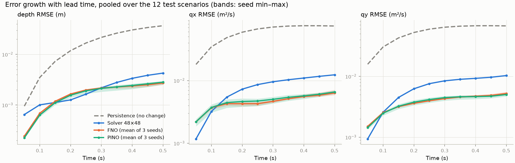
Figure 4 shows something the averages hide. The solver is more accurate at early times: up to about 0.1 s for discharge, and from about 0.15 to 0.3 s for depth. Its error then grows steadily, as numerical diffusion accumulates. The operators’ error rises quickly at first and then levels off. The neural advantage therefore comes from the later part of the horizon. Chapter 5 tests whether it persists over a five times longer horizon: it does, by a smaller margin.
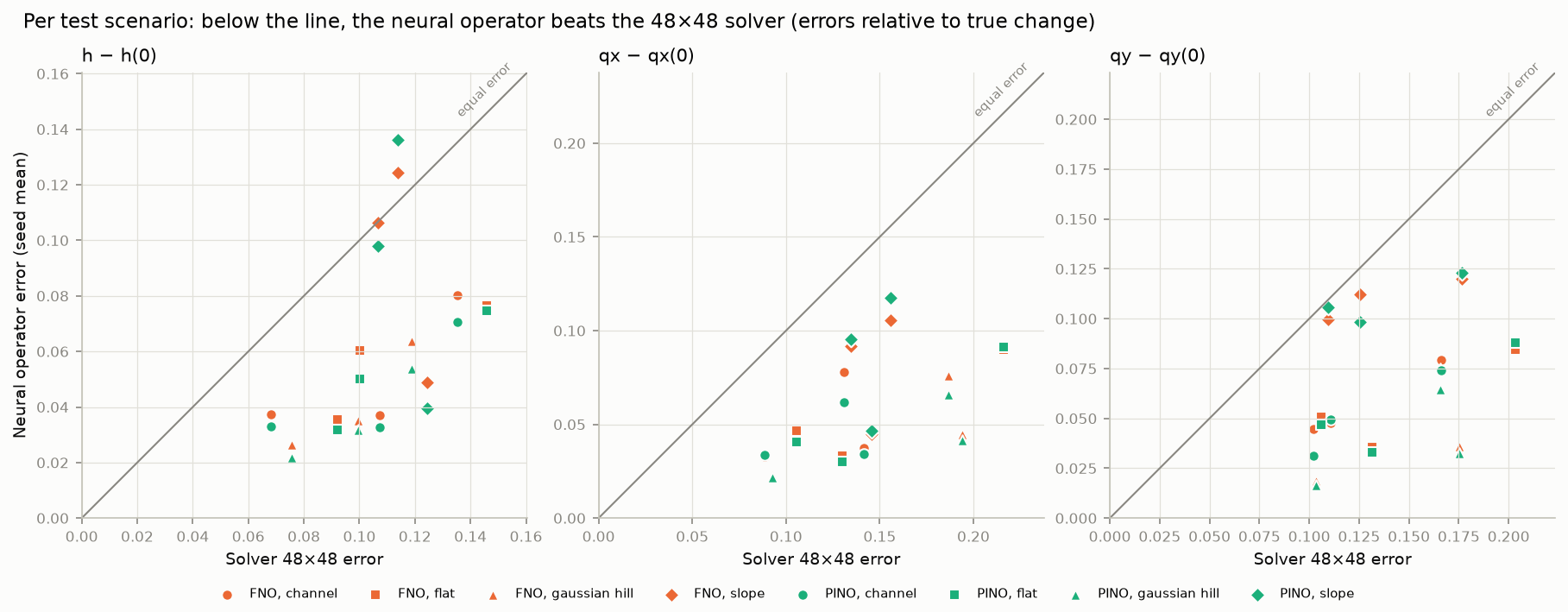
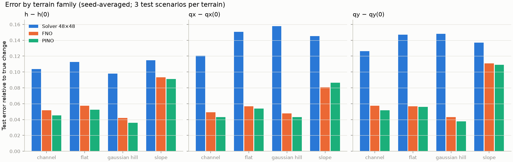
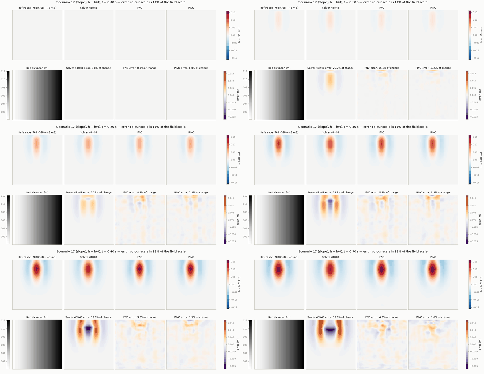
Figure 5 and Figure 6 show that the operators beat the solver in 11 of the 12 test scenarios in depth, and in all 12 in discharge. The planar slope is the hardest family. There the operators’ errors are about twice those on other terrain, and their advantage over the solver shrinks: about 20% in depth and \(q_y\), against roughly 50% on flat, hill and channel terrain. The slope is the only family in which the depth, and therefore the wave speed \(\sqrt{gh}\), changes steadily across the whole basin: rings travel faster on the deep side than on the shallow side and become lopsided. Three test scenarios per family are a thin basis for such a different regime.
5.3 What the errors look like
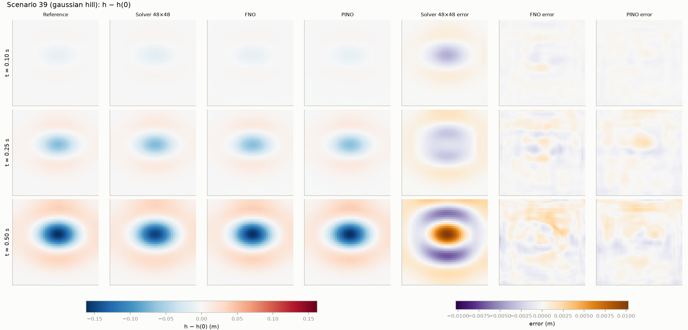
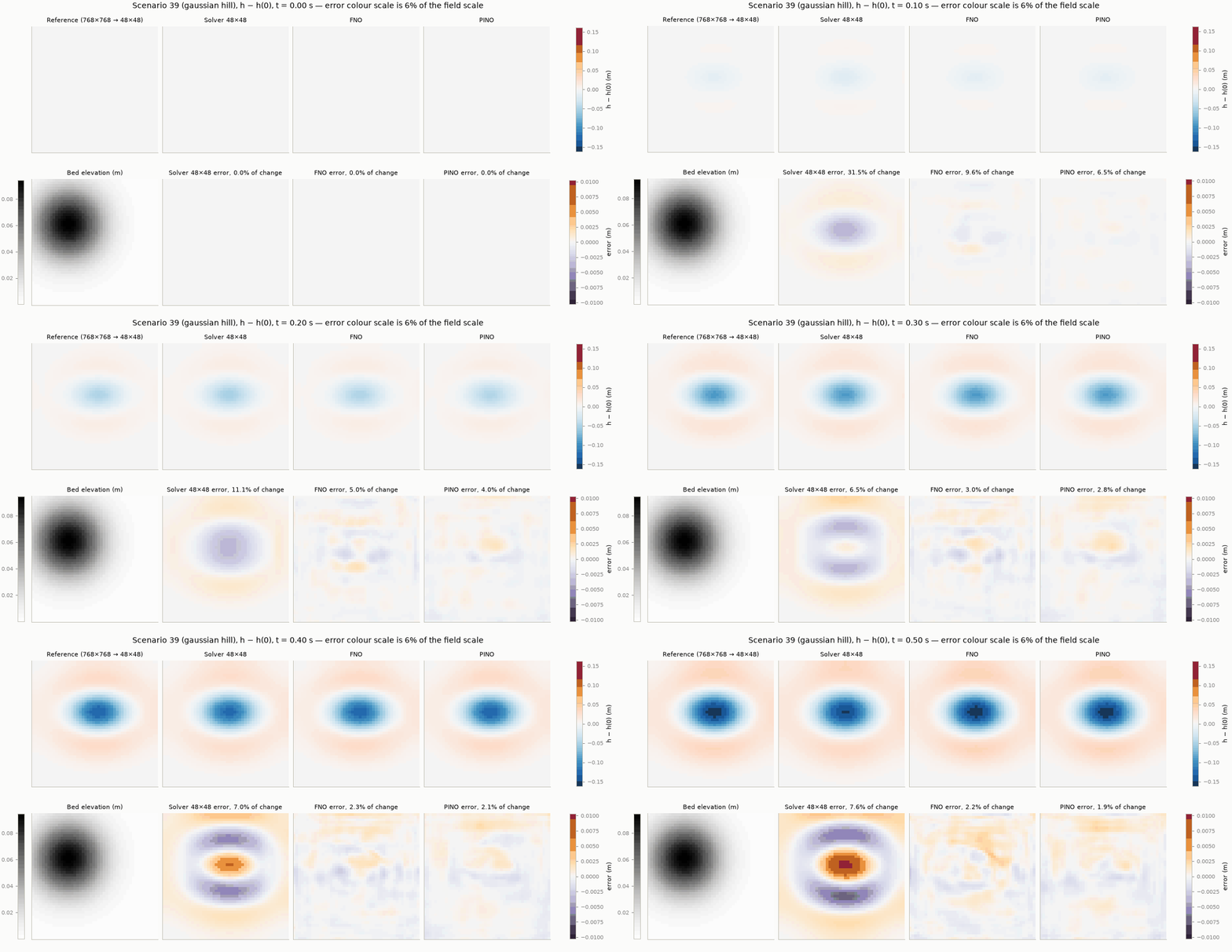
The animations below run from \(t = 0\) to \(0.5\) s. In each, the top row shows the reference, the solver, the FNO and the PINO. The bottom row shows the bed and each method’s error, on a colour scale several times narrower than the fields.
5.4 Choices made along the way
Each of these was judged on validation scenarios, never on test scenarios:
- Model size made little difference. Widths of 24, 32 and 48 channels gave almost the same validation error, about 0.20 without augmentation, while the training error kept falling. The network was overfitting: fitting the 56 training scenarios ever more closely without improving on new ones. It was not short of capacity.
- Symmetry augmentation was the largest single gain. It cut validation error from about 0.20 to 0.05. It comes from physical knowledge applied to the data, not to the loss.
- Data scarcity hurts. With 14 labelled scenarios the test error rises to about 0.20, and varies strongly with the seed (Figure 3, right).
5.5 Resolution and boundaries
Because the Fourier weights are tied to wavenumbers, not to grid cells, the same trained network can be run on 96 × 96 versions of the test scenarios, a grid it has never seen, without retraining. This is called zero-shot evaluation:
| model | grid | depth anomaly err | qx change err | qy change err | wall-band RMSE | interior RMSE |
|---|---|---|---|---|---|---|
| FNO | 48 x 48 (training grid) | 0.0610 | 0.0586 | 0.0670 | 0.0052 | 0.0051 |
| FNO | 96 x 96 (zero-shot) | 0.0637 | 0.0600 | 0.0691 | 0.0063 | 0.0052 |
| PINO | 48 x 48 (training grid) | 0.0562 | 0.0567 | 0.0636 | 0.0051 | 0.0050 |
| PINO | 96 x 96 (zero-shot) | 0.0589 | 0.0587 | 0.0663 | 0.0059 | 0.0051 |
| FNO, padded (seed 2026, 192 x 192 reference) | 48 x 48 | 0.0596 | 0.0583 | 0.0638 | 0.0051 | 0.0049 |
| FNO, no padding (seed 2026, 192 x 192 reference) | 48 x 48 | 0.0522 | 0.0497 | 0.0514 | 0.0051 | 0.0041 |
- Zero-shot resolution. Error rises only slightly at 96 × 96, mostly in the band next to the walls.
- Padding. The padding test was a single run on the 192 × 192 reference, so the table compares it with the padded run of the same seed and reference. The unpadded run was better overall, by about 10–20%, with the same wall-band error. Because waves barely reach the walls within 0.5 s (Chapter 1, table of characteristic scales), this benchmark is a weak test of boundary treatment. A design choice that sounds necessary is not automatically beneficial; it must be measured.
6 Limitations
The FNO was trained and tested on one synthetic distribution: four smooth terrain families, fully wet, a fixed 10 m basin and a 0.5 s horizon. Chapter 5 adds a test over 2.5 s. Other domain sizes, wet/dry fronts and field data are untested. Its accuracy is measured against a numerical reference that has its own error of about 1%.
- Operator learning trains a network \(\mathcal G_\theta\) to map a whole scenario (bed and initial state) to its solution, Equation \(\eqref{eq-operator}\). New scenarios then cost one forward pass.
- DeepONet combines a branch and a trunk network, Equation \(\eqref{eq-deeponet}\). The FNO mixes information globally through learned multiplications in Fourier space, Equation \(\eqref{eq-fourier-layer}\).
- Fourier layers assume periodicity, so walls need care such as padding, and that care must be tested.
- Predicting the change, Equation \(\eqref{eq-change-param}\), symmetry augmentation, Equation \(\eqref{eq-mirror}\), and refined training data were the choices that made the FNO accurate.
- On held-out scenarios the FNO is about 16× better than persistence and about 45–60% more accurate than a solver at the same resolution. It is worse than the solver at early times, and its lead is smallest on sloping terrain.
- Why would splitting individual time snapshots, rather than whole scenarios, between training and test give misleading results?
- In Equation \(\eqref{eq-mirror}\), why must \(q_x\) change sign but \(q_y\) not?
- Using Figure 4, at what times would you rather use the coarse solver than the FNO?
- The FNO beat the 48 × 48 solver. Does that mean it is “more accurate than numerical simulation”? Explain.
- Why might the slope terrain be harder for the operator to learn?