Physics-informed neural operators
Adding the governing equations to operator training
By the end of this chapter you should be able to:
- Explain what a physics-informed neural operator (PINO) adds to a data-trained operator, and what it does not change.
- Write a discrete shallow-water residual on a grid, and explain why it uses a well-balanced form, central differences and a Crank–Nicolson time step.
- Explain the trade-off controlled by the physics weight \(\lambda\), and how to choose it without touching test data.
- Explain why physics losses can use unlabelled scenarios, and when this matters most.
- Interpret the PINO results honestly, including small effects and single-seed results.
1 Why combine operators and physics?
The FNO of Chapter 3 learns only from examples. Nothing in its loss says that mass must be conserved or that water should flow downhill. Within the training distribution this may not matter, but two weaknesses remain:
- The predictions need not obey the equations. They can be accurate on average and still contain physically impossible patterns.
- Every training example needs a simulation. When simulations are expensive, labelled data are scarce, and Chapter 3 showed that the FNO degrades sharply with 14 scenarios instead of 56.
A physics-informed neural operator (PINO) (Li et al. 2024) adds the residual of the governing equations (how far a prediction is from satisfying them, Chapter 2) to the operator’s training loss, just as a PINN does for a single solution:
\[ \begin{equation} \mathcal L_{\text{PINO}} = \mathcal L_{\text{data}} + \lambda\, \big(\mathcal L_{\text{PDE}} + \mathcal L_{\text{wall}}\big). \label{eq-pino} \end{equation} \]
Here \(\mathcal L_{\text{data}}\) is the FNO’s loss of Chapter 3, the error relative to the change; \(\mathcal L_{\text{PDE}}\) and \(\mathcal L_{\text{wall}}\) penalise breaking the equations and letting water through the walls; and the weight \(\lambda\) sets how much the physics counts.
1.1 PINO is a training method, not a new architecture
The seminar’s PINO is exactly the FNO of Chapter 3: same architecture, data, split, augmentation, epochs, seeds and checkpoint selection. Only the loss changes. Any difference in results is therefore caused by the physics terms. It also means the physics loss does not remove the architecture’s limitations, such as Fourier layers and non-periodic walls.
2 From PINN residual to PINO residual
A PINN is a function of continuous \((x, y, t)\), so automatic differentiation gives its derivatives exactly. An FNO outputs values on a 48 × 48 grid at ten times. Its derivatives must be approximated on that grid, with finite differences: the difference between neighbouring values divided by their spacing. Three choices make this residual faithful.
2.1 Space: central differences in a well-balanced form
Write the right-hand side of the conservative SWE (Chapter 1, conservative form) as a tendency \(\mathbf T(\mathbf U) = \partial \mathbf U / \partial t\):
\[ \begin{equation} \mathbf T(\mathbf U) = \begin{pmatrix} -\,\delta_x q_x - \delta_y q_y \\[2pt] -\,\delta_x\!\big(q_x^2/h\big) - \delta_y\!\big(q_x q_y/h\big) - g h\, \delta_x (h + z_b) \\[2pt] -\,\delta_x\!\big(q_x q_y/h\big) - \delta_y\!\big(q_y^2/h\big) - g h\, \delta_y (h + z_b) \end{pmatrix}, \label{eq-tendency} \end{equation} \]
where \(\delta_x\) is the central difference \((f_{i+1} - f_{i-1}) / 2\Delta x\), which uses the neighbours on both sides. It is second-order accurate: its error shrinks with the square of the cell size.
The pressure and bed terms are combined into \(g h\, \nabla(h + z_b) = g h\, \nabla \eta\), the well-balanced form of Chapter 1. For a lake at rest, \(\eta\) is constant, so this term is exactly zero on the grid. Differencing \(\tfrac12 g h^2\) and \(z_b\) separately would leave a small spurious force over every hill, and the loss would then push the model away from rest.
At the walls, a cell has no neighbour on one side. Imaginary ghost cells just outside the wall supply it, as a mirror image of the cells inside. Depth, bed and the discharge along the wall are mirrored unchanged. The normal discharge is reflected with its sign flipped, so the flow through the wall is zero.
2.2 Time: Crank–Nicolson between output frames
The outputs are 0.05 s apart, and the known initial state is frame 0. Between consecutive frames, the residual compares the actual change with the average tendency at the two ends. This is the trapezoidal or Crank–Nicolson rule:
\[ \begin{equation} \mathbf R^{n+\frac12} = \frac{\mathbf U^{n+1} - \mathbf U^{n}}{\Delta t} - \frac12\Big(\mathbf T(\mathbf U^{n+1}) + \mathbf T(\mathbf U^{n})\Big),\qquad n = 0, \dots, 9. \label{eq-cn} \end{equation} \]
This is second-order accurate in time. Including \(n = 0\) anchors the first prediction to the true initial state.
2.3 The loss terms
The residual is in physical units, which differ between variables. Each component is divided by its typical tendency, \(s_i / T\): the training-set change scale \(s_i\) from Chapter 3 over the horizon \(T\). Then
\[ \begin{equation} \mathcal L_{\text{PDE}} = \Big\langle \big(\mathbf R^{n+\frac12}_i\, T / s_i\big)^2 \Big\rangle,\qquad \mathcal L_{\text{wall}} = \Big\langle \big(q_n^{\text{wall}} / \bar s_q\big)^2 \Big\rangle, \label{eq-physics-loss} \end{equation} \]
where:
- angle brackets average over cells, times, variables and scenarios;
- \(q_n^{\text{wall}}\) is the normal discharge extrapolated to each wall, which should be zero;
- \(\bar s_q\) is the mean discharge change scale.
The initial condition needs no loss term, because it is exact by construction (Chapter 3, “predict the change”).
Ramping. In the first epochs the network output is random, and a strong physics loss would dominate. The physics weight is therefore multiplied by a ramp from 0 to 1 over the first 20% of training.
The tables report a PDE residual: the root-mean-square of Equation \(\eqref{eq-cn}\) over all cells and frames, with each variable divided by its typical change \(s_i\). Its value means little on its own; compare it with that of the accurate labels.
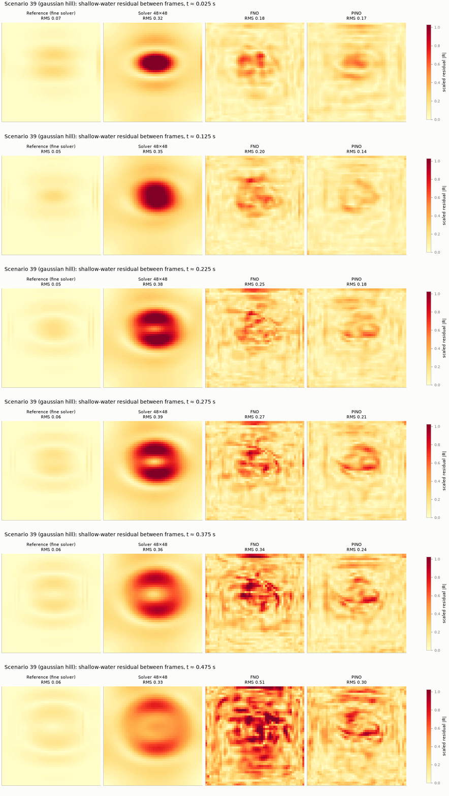
The labels come from a 768 × 768 finite-volume solver, averaged to 48 × 48. Evaluated with Equation \(\eqref{eq-cn}\) on the 48 × 48 grid, they have a residual of about 0.14 on the test scenarios, not 0. The FNO’s predictions have about 0.63. Pushing the residual all the way to zero would therefore pull the model away from the true solution. This is why \(\lambda\) cannot simply be made large.
3 Choosing the physics weight
The weight \(\lambda\) was chosen on validation scenarios from {0, 0.003, 0.03, 0.3, 1, 3}, with a single seed. This search was made with the earlier 192 × 192 reference; the chosen weight was then kept for the 768 × 768 runs.
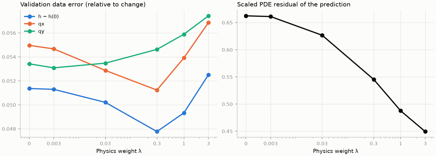
| model | labelled | seeds | depth anomaly err | qx change err | qy change err | depth RMSE (m) | qx RMSE (m²/s) | qy RMSE (m²/s) | mass err | PDE residual | wall normal q (m²/s) |
|---|---|---|---|---|---|---|---|---|---|---|---|
| λ = 0 | 56 | 1 | 0.051 | 0.055 | 0.053 | 0.0013 | 0.0033 | 0.0035 | 8.6e-05 | 0.662 | 0.0046 |
| λ = 0.003 | 56 | 1 | 0.051 | 0.055 | 0.053 | 0.0013 | 0.0033 | 0.0035 | 8.8e-05 | 0.661 | 0.0044 |
| λ = 0.03 | 56 | 1 | 0.050 | 0.053 | 0.053 | 0.0013 | 0.0032 | 0.0035 | 1.0e-04 | 0.627 | 0.0040 |
| λ = 0.3 | 56 | 1 | 0.048 | 0.051 | 0.055 | 0.0012 | 0.0030 | 0.0036 | 1.0e-04 | 0.545 | 0.0033 |
| λ = 1 | 56 | 1 | 0.049 | 0.054 | 0.056 | 0.0012 | 0.0032 | 0.0036 | 7.2e-05 | 0.488 | 0.0024 |
| λ = 3 | 56 | 1 | 0.053 | 0.057 | 0.057 | 0.0013 | 0.0033 | 0.0036 | 9.5e-05 | 0.449 | 0.0023 |
Figure 1 shows the trade-off typical of physics-informed training. A little physics helps the data fit, because the two objectives agree. Too much physics hurts it, because they begin to compete: recall that the labels themselves do not have zero residual. We chose \(\lambda = 0.3\) for both terms.
The differences are small, and the gain in \(q_y\) is absent. With a single seed per value, the optimum is only roughly located.
4 Results
4.1 With plenty of labelled data
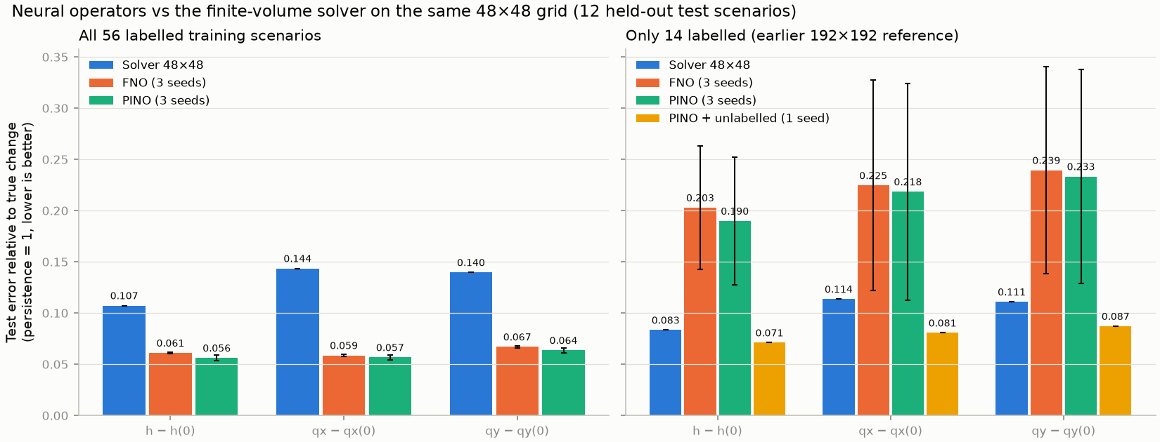
With all 56 labelled training scenarios, the PINO is compared with the FNO on the 12 test scenarios, with three seeds each (Table 2).
| model | labelled | seeds | depth anomaly err | qx change err | qy change err | depth RMSE (m) | qx RMSE (m²/s) | qy RMSE (m²/s) | mass err | PDE residual | wall normal q (m²/s) |
|---|---|---|---|---|---|---|---|---|---|---|---|
| Persistence (no change) | - | 1 | 1.000 | 1.000 | 1.000 | 0.0212 | 0.0577 | 0.0523 | 0.0e+00 | 5.365 | 0.0000 |
| Finite-volume solver, 48 x 48 | - | 1 | 0.107 | 0.144 | 0.140 | 0.0023 | 0.0081 | 0.0070 | 1.1e-07 | 0.496 | 0.0003 |
| FNO (data only) | 56 | 3 | 0.061 ± 0.001 | 0.059 ± 0.001 | 0.067 ± 0.001 | 0.0015 ± 0.0000 | 0.0036 ± 0.0001 | 0.0034 ± 0.0001 | 1.4e-04 ± 1.2e-05 | 0.635 ± 0.003 | 0.0049 ± 0.0002 |
| PINO (data + physics) | 56 | 3 | 0.056 ± 0.003 | 0.057 ± 0.002 | 0.064 ± 0.002 | 0.0014 ± 0.0001 | 0.0036 ± 0.0002 | 0.0032 ± 0.0002 | 1.5e-04 ± 1.5e-05 | 0.513 ± 0.024 | 0.0037 ± 0.0002 |
- The PINO is slightly better on every data error, by about 3–8%, and its PDE residual is about 19% lower. The differences are one to two seed standard deviations: consistent, but small.
- Mass error does not change, because volume is already close to conserved.
- Figure 3 (left panel) and the time and terrain plots in Chapter 3 show the FNO and PINO almost on top of each other. With 56 labelled scenarios, the data already pin down the solution; physics adds little.
Figure 2 shows where each model violates the equations, over the 0.5 s of one test scenario. The fine solver’s own residual is low but not zero: it was computed on a finer grid, so it does not exactly satisfy the 48 × 48 equations. The 48 × 48 solver concentrates its residual on the moving wave, where its numerical diffusion acts. The FNO’s residual is noisy and spread over the basin. The PINO’s is visibly cleaner, which is exactly what its physics loss rewards.
4.2 With scarce labelled data
Now only 14 labelled scenarios are used: a quarter of the training set, with the same number from each terrain family. Training runs for the same number of optimisation steps as before. These runs were made with the earlier 192 × 192 reference, so they are compared with the 48 × 48 solver scored against that same reference.
| model | labelled | seeds | depth anomaly err | qx change err | qy change err | depth RMSE (m) | qx RMSE (m²/s) | qy RMSE (m²/s) | mass err | PDE residual | wall normal q (m²/s) |
|---|---|---|---|---|---|---|---|---|---|---|---|
| Finite-volume solver, 48 x 48 | - | 1 | 0.083 | 0.114 | 0.111 | 0.0018 | 0.0062 | 0.0055 | 1.0e-07 | 0.505 | 0.0003 |
| FNO, 14 labelled | 14 | 3 | 0.203 ± 0.060 | 0.225 ± 0.103 | 0.239 ± 0.101 | 0.0039 ± 0.0006 | 0.0098 ± 0.0017 | 0.0094 ± 0.0020 | 9.8e-04 ± 6.9e-04 | 1.480 ± 0.151 | 0.0104 ± 0.0029 |
| PINO, 14 labelled | 14 | 3 | 0.190 ± 0.062 | 0.218 ± 0.106 | 0.233 ± 0.105 | 0.0036 ± 0.0006 | 0.0095 ± 0.0019 | 0.0092 ± 0.0022 | 9.5e-04 ± 6.7e-04 | 1.308 ± 0.185 | 0.0093 ± 0.0034 |
| PINO, 14 labelled + 240 unlabelled | 14 | 1 | 0.071 | 0.081 | 0.087 | 0.0016 | 0.0050 | 0.0042 | 3.1e-04 | 0.605 | 0.0039 |
- Physics on the same 14 scenarios barely helps. The gain is far smaller than the variation between seeds. The labels already constrain the solution on those inputs.
- Physics on new inputs helps a lot. A physics loss needs only inputs: a bed and an initial state, with no solver run. Adding 240 unlabelled scenarios from the same generator cuts the error to about a third, close to the FNO trained on all 56 labelled scenarios.
- This is a single seed and needs replication before it is treated as established.
- This is not extrapolation. The unlabelled scenarios come from the training distribution. The result shows physics replacing simulations, not physics enabling predictions for new kinds of scenario.
This is the regime where physics-informed training earns its cost: when simulations are expensive and inputs are cheap.
5 Limitations
- The residual is a grid version of the SWE without friction or viscosity, on a 48 × 48 grid, and the labels do not satisfy it exactly.
- The scarce-data experiment was run only over 0.5 s, with smooth, fully wet flow. Chapter 5 tests a 2.5 s horizon, for which the weight \(\lambda\) had to be chosen again.
- \(\lambda\) was tuned on one seed, with the PDE and wall weights kept equal.
- Physics-informed training was not tested on out-of-distribution scenarios, ones unlike any in training, where it might help or hurt.
- A PINO is a neural operator trained with an extra physics loss, Equation \(\eqref{eq-pino}\). The architecture is unchanged.
- On a grid, the residual uses finite differences: central differences in a well-balanced form, Equation \(\eqref{eq-tendency}\), and a Crank–Nicolson step between output frames, Equation \(\eqref{eq-cn}\).
- The physics weight trades data fit against residual. Here the best validation weight was \(\lambda = 0.3\), and it was chosen without touching test data.
- With 56 labelled scenarios, physics gives a small, consistent gain (about 3–8% in error, 19% in residual).
- Physics pays off when labels are scarce and unlabelled inputs are added. In one seed, 240 unlabelled scenarios cut the error threefold.
- Why does the PINO residual use finite differences while the PINN residual used automatic differentiation?
- What would happen to a lake at rest over a hill if the pressure and bed terms were differenced separately?
- Why can’t \(\lambda\) be increased until the residual is zero?
- Why do unlabelled scenarios help a PINO but would be useless to an FNO?
- The PINO+unlabelled result is from one seed. What would you need to see before relying on it?