flowchart LR
  A["1. sample scenarios:<br/>bed, initial state"] --> B["2. fine solver<br/>768 × 768"]
  B --> C["3. average to<br/>48 × 48"]
  C --> D["4. train FNO / PINO"]
  D -->|"trained model"| F["one forward pass<br/>(about 6 ms)"]
  E["new scenario:<br/>bed, initial state"] --> F
  F --> G["depth and discharge<br/>at 10 times"]
A fast shallow-water emulator
Putting it together: accuracy, cost and trust
Learning objectives
By the end of this chapter you should be able to:
- Describe the full emulation workflow: generate simulations, train, then predict new scenarios.
- Define the metrics used to evaluate an emulator, and explain what each one can and cannot reveal.
- Separate training cost from inference cost, and estimate when an emulator pays for itself.
- Run the end-to-end demonstration and the comparison plots in Docker.
- Explain what changes when the prediction horizon is extended, and why a physics weight may need to be chosen again.
- State clearly what this emulator demonstrates, and what it does not.
1 The emulation workflow
An emulator moves the cost of simulation from when you need an answer to before you need it:
Steps 1–4 form the offline phase: expensive, but done once. Everything to the right of the trained model is the online phase, or inference: using the trained model to predict. It is repeated for every new scenario, and it is cheap. That suits tasks that need many predictions: ensembles (many runs with varied inputs, to capture uncertainty), sensitivity studies, optimisation and real-time “what-if” analysis.
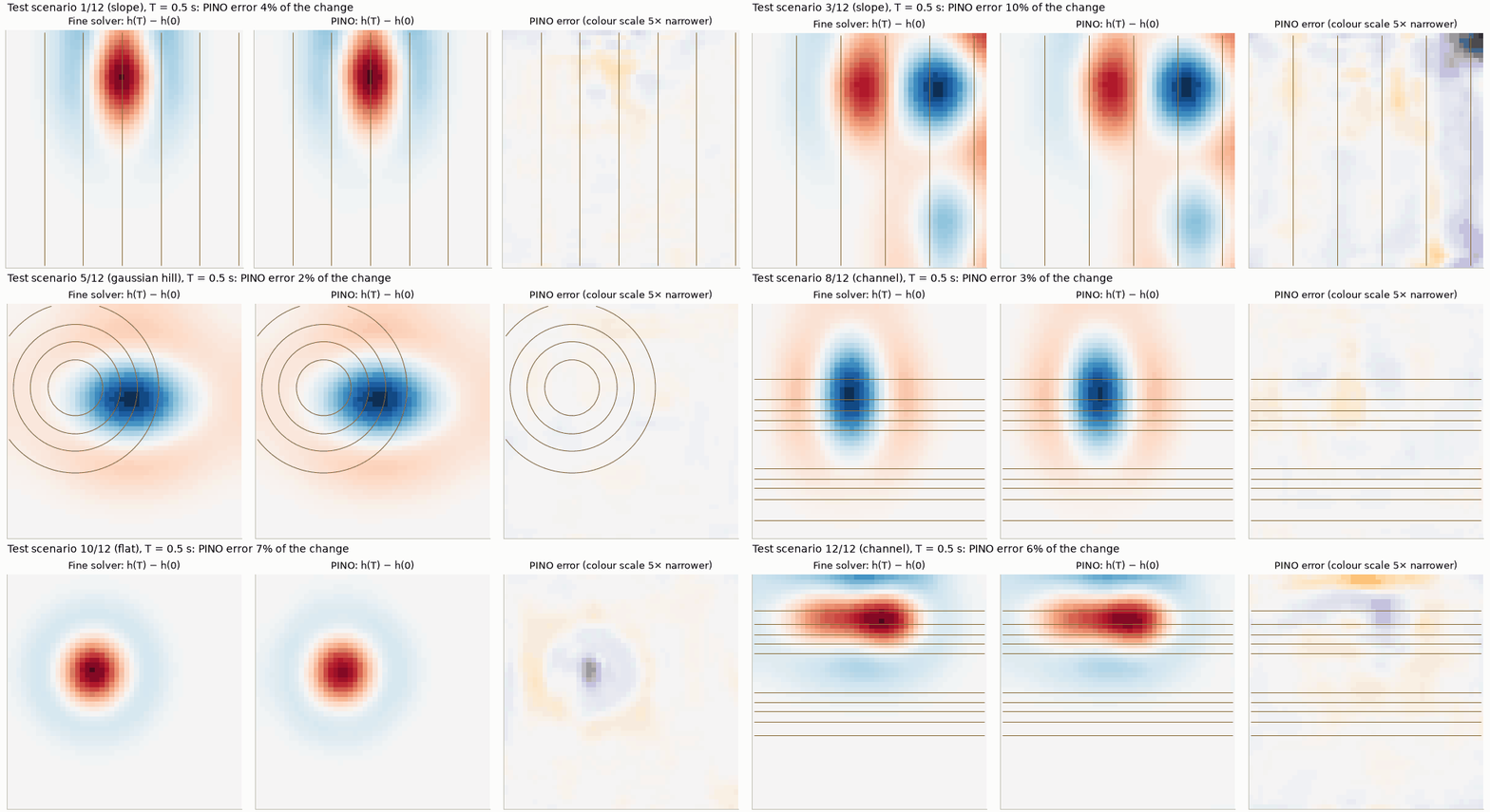
Figure 1 shows the online phase on all 12 held-out test scenarios, which the model never saw during training. Each prediction takes about 6 ms, against about 110 s for the 768 × 768 reference solver (one CPU thread).
2 How we evaluate an emulator
A plausible-looking picture is not evidence. Every model, including the solver baseline, is scored on the same 12 held-out test scenarios with the same metrics. Each scenario counts equally.
Error relative to the change (the headline metric, as in Chapters 2–4):
\[ \begin{equation} e_q = \frac{\|q_{\text{pred}} - q_{\text{ref}}\|_2}{\|q_{\text{ref}} - q_0\|_2},\qquad q \in \{h, q_x, q_y\}. \label{eq-skill} \end{equation} \]
Persistence scores 1 and a perfect model 0. It answers the question “how much of the change did we get wrong?”
Root-mean-square error in physical units, metres for depth and m²/s for discharge:
\[ \begin{equation} \mathrm{RMSE}_q = \sqrt{\big\langle (q_{\text{pred}} - q_{\text{ref}})^2 \big\rangle}, \label{eq-rmse} \end{equation} \]
where the angle brackets average over all cells and output times.
Mass error, the largest relative drift in total water volume \(V(t) = \sum h\,\Delta x\,\Delta y\):
\[ \begin{equation} e_{\text{mass}} = \max_t \frac{|V(t) - V(0)|}{V(0)}. \label{eq-mass-error} \end{equation} \]
A walled basin must conserve volume exactly (Chapter 1).
PDE residual: how far the prediction is from satisfying the shallow-water equations on the grid, measured as in Chapter 4. It does not need the reference, so it can also be computed for a new scenario where no reference exists. Compare it with the residual of the accurate labels, which is small but not zero.
Wall flux: the discharge through the walls, which should be zero.
Wall band versus interior error: RMSE in the two cells next to each wall, against the rest. This exposes boundary artefacts.
Inference time per scenario: measured on one CPU thread (one processor core) on an otherwise idle machine, excluding the first call, which includes one-off set-up. It is reported with the hardware, the grid and the batch size, the number of scenarios evaluated together.
3 Try it yourself
The hands-on folder (see Before the seminar) contains the dataset and both trained models, so nothing has to be generated or trained first.
- Notebook 3 runs the 48 × 48 solver live on the 12 test scenarios, runs both operators, and reports the errors, mass conservation, PDE residual and timings defined above.
- Notebook 4 uses the PINO for an ensemble of 200 what-if runs, compares it with the solver, and trains a small FNO from scratch.
Building everything from scratch takes far longer. The 768 × 768 data take several hours on a laptop, even with 8 parallel workers, and training each model takes about 25–50 minutes on a laptop CPU. A 192 × 192 reference instead takes a few minutes, at the cost of labels that are about 3.5–4.5% off rather than 1%.
4 Accuracy and cost
| Method | seconds per scenario | relative to 768 x 768 solver |
|---|---|---|
| Finite-volume solver, 768 x 768 (the reference) | 108.8053 | 1x |
| Finite-volume solver, 192 x 192 | 1.1561 | 94x faster |
| Finite-volume solver, 48 x 48 | 0.0314 | 3466x faster |
| FNO or PINO, 48 x 48, one scenario at a time | 0.0059 | 18594x faster |
| FNO or PINO, 48 x 48, 12 scenarios per batch | 0.0046 | 23570x faster |
CPU: 13th Gen Intel(R) Core(TM) i9-13900H; one thread; PyTorch 2.15.0+cpu.
4.1 When does an emulator pay for itself?
Training is not free. The cost of building the emulator is the time to simulate the training scenarios plus the time to train:
- about 8,700 s (2.4 h) for 80 simulations on 768 × 768 cells, one thread each;
- about 1,500 s of training, on 6 threads.
Each later prediction saves the difference between a fine solve and a network evaluation. The break-even number of predictions, after which the emulator has saved more time than it cost, is
\[ \begin{equation} N^\ast \approx \frac{T_{\text{data}} + T_{\text{train}}}{t_{\text{solver}} - t_{\text{emulator}}} \approx \frac{8700 + 1500\ \text{s}}{109 - 0.006\ \text{s}} \approx 90. \label{eq-breakeven} \end{equation} \]
Here \(T_{\text{data}}\) and \(T_{\text{train}}\) are the one-off costs, and \(t_{\text{solver}}\) and \(t_{\text{emulator}}\) are the costs of one prediction by each method.
Against the 768 × 768 reference, the emulator pays for itself after about a hundred predictions. The number is rough, because training used several threads while the solvers and inference were timed on one.
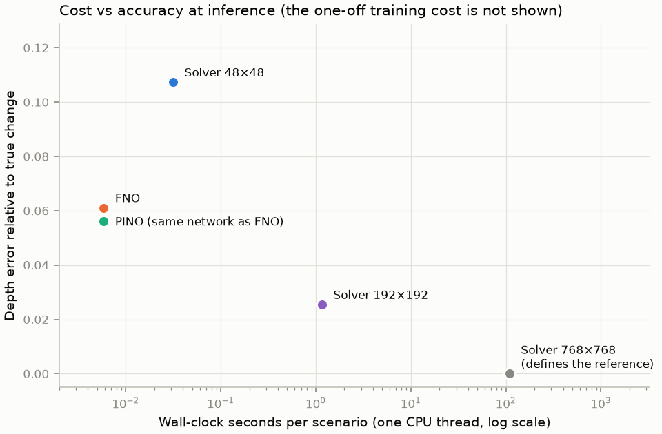
The fair comparison is less flattering. Nobody needs the 768 × 768 solver to match the emulator’s accuracy: a 192 × 192 solver is already about 2.4× more accurate than the FNO (Figure 2), and it takes about 1.2 s. Against that solver, \(N^\ast \approx 10200 / 1.15 \approx 9000\) predictions. An emulator is worthwhile when you need many thousands of predictions, or each one immediately, and can accept its error. The more expensive the solver for a given accuracy, the smaller \(N^\ast\).
5 Where to be careful
The previous chapters found several regimes where the emulator is weaker than its average score suggests:
- Early times. The coarse solver is more accurate than the operators up to about 0.1 s in discharge, and from about 0.15 to 0.3 s in depth (Chapter 3, error over time).
- Sloping terrain. On the slope family the operators’ errors are about twice those on other terrain, and their lead over the solver shrinks to about 20% (Chapter 3).
- Few training simulations. With 14 instead of 56 labelled scenarios, the error triples, unless the physics loss is also given unlabelled scenarios (Chapter 4, an experiment on the earlier 192 × 192 reference).
How would you know, for a new scenario, whether to trust the prediction? The reference is not available then, but the PDE residual and the mass error are. A prediction with an unusually large residual is a warning sign. Using it as a formal trust indicator is a natural next step, and it has not been tested here.
6 Longer horizons
Everything so far used a 0.5 s horizon. In that time a wave travels about 2 m, so it barely reaches the walls (Chapter 1, table of characteristic scales). Reflections, interference and terrain steering, the behaviour that makes basin flow hard, lie mostly outside the test. To probe them, the same 80 scenarios were run five times longer, to \(T = 2.5\) s, about the time a wave takes to cross the basin (Chapter 1, the longer sample runs). Everything else is unchanged: the same splits, the same 768 × 768 reference averaged to 48 × 48, and the same metrics.
The network is also unchanged, except for its output layer: it now predicts 50 frames, 150 output channels instead of 30. Both models were trained for 2000 epochs instead of 1000, with one seed each. At 0.5 s the spread between seeds was about 3–5% of the error, so smaller differences between FNO and PINO here are not conclusive.
6.1 The physics weight had to be chosen again
In the physics loss of Chapter 4, the residual of each variable is multiplied by \(T/s_i\): the horizon divided by that variable’s typical change. The horizon grew 5×, but the typical changes grew far less: 1.8× in depth and hardly at all in discharge. The same residual therefore costs about 8–22× more in the loss. With the 0.5 s weight \(\lambda = 0.3\), the physics term swamped the data: the validation depth error was 0.48, four times the FNO’s. The weight was therefore searched again on the validation scenarios (Table 2).
| model | labelled | seeds | depth anomaly err | qx change err | qy change err | depth RMSE (m) | qx RMSE (m²/s) | qy RMSE (m²/s) | mass err | PDE residual | wall normal q (m²/s) |
|---|---|---|---|---|---|---|---|---|---|---|---|
| λ = 0 | 56 | 1 | 0.117 | 0.220 | 0.183 | 0.0049 | 0.0123 | 0.0123 | 6.2e-04 | 1.605 | 0.0127 |
| λ = 0.003 | 56 | 1 | 0.098 | 0.204 | 0.175 | 0.0041 | 0.0114 | 0.0117 | 4.8e-04 | 0.868 | 0.0119 |
| λ = 0.012 | 56 | 1 | 0.118 | 0.235 | 0.219 | 0.0050 | 0.0134 | 0.0148 | 6.2e-04 | 0.717 | 0.0106 |
| λ = 0.03 | 56 | 1 | 0.265 | 0.447 | 0.712 | 0.0111 | 0.0252 | 0.0485 | 1.4e-03 | 0.721 | 0.0086 |
| λ = 0.3 | 56 | 1 | 0.479 | 0.867 | 0.892 | 0.0203 | 0.0495 | 0.0612 | 3.4e-04 | 0.650 | 0.0037 |
Only a narrow window helps. At \(\lambda = 0.003\) the depth error drops by about 16% and the residual nearly halves. At \(\lambda = 0.012\) the gain is gone, and from 0.03 upwards training fails. The weight chosen at one horizon did not carry over to another. Whenever the setting changes, the weight must be chosen again on validation data.
6.2 Results
| model | labelled | seeds | depth anomaly err | qx change err | qy change err | depth RMSE (m) | qx RMSE (m²/s) | qy RMSE (m²/s) | mass err | PDE residual | wall normal q (m²/s) |
|---|---|---|---|---|---|---|---|---|---|---|---|
| Persistence (no change) | - | 1 | 1.000 | 1.000 | 1.000 | 0.0370 | 0.0602 | 0.0556 | 0.0e+00 | 5.039 | 0.0000 |
| Finite-volume solver, 48 x 48 | - | 1 | 0.191 | 0.403 | 0.385 | 0.0069 | 0.0230 | 0.0204 | 1.2e-07 | 0.269 | 0.0002 |
| FNO (data only) | 56 | 1 | 0.126 | 0.226 | 0.217 | 0.0047 | 0.0138 | 0.0113 | 4.3e-04 | 1.289 | 0.0101 |
| PINO (data + physics, λ = 0.003) | 56 | 1 | 0.117 | 0.207 | 0.205 | 0.0043 | 0.0127 | 0.0107 | 4.5e-04 | 0.836 | 0.0103 |
- The operators still beat the coarse solver. They have about 35–40% less error in depth and 45–50% less in discharge, on every terrain family. The advantage is not an artefact of the short horizon.
- But the advantage is smaller. Compared with 0.5 s, every method’s error is about twice as large in depth and three to four times as large in discharge. The FNO’s lead over the solver shrinks from about 43% to 34% in depth, and from about 59% to 44% in discharge.
- The PINO is 5–8% better than the FNO in all three variables. Its residual is a third lower, 0.84 against 1.29. Both are still far above the labels’ own residual of 0.12 and the solver’s 0.27, much further than at 0.5 s.
- The walls are now a weakness. The operators let about 0.01 m²/s through the walls, 50 times the solver’s leak and twice their own at 0.5 s. At \(\lambda = 0.003\) the wall penalty is too weak to change this. It matters more now, because waves do reach the walls.
- Slope remains the hardest family. There the operators beat the solver by about 20% in depth, against 35–46% on the other three.
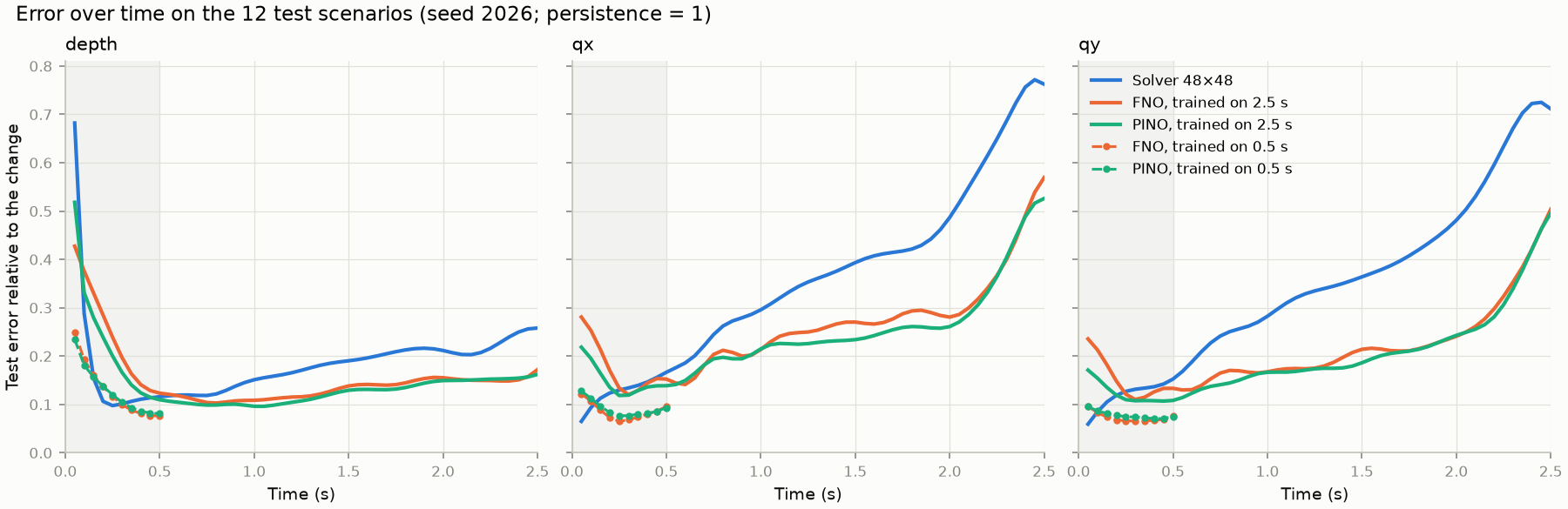
Figure 4 shows how the errors develop:
- The coarse solver is ahead early on, for longer than before. It is better until about 0.5 s in depth and about 0.2–0.25 s in discharge, compared with about 0.3 s and 0.1 s at 0.5 s. After that its error grows steadily, while the operators’ error grows more slowly.
- A long horizon costs accuracy early on. Over the first 0.5 s, the models trained on 2.5 s are clearly worse than those trained on 0.5 s: at \(t = 0.5\) s, the FNO’s depth error is 0.12 instead of 0.08. A likely reason: the same network must now fit 50 frames instead of 10, and the later frames, which change more, dominate its loss. If early times matter, a separate short-horizon model, or a larger network, is the better choice.
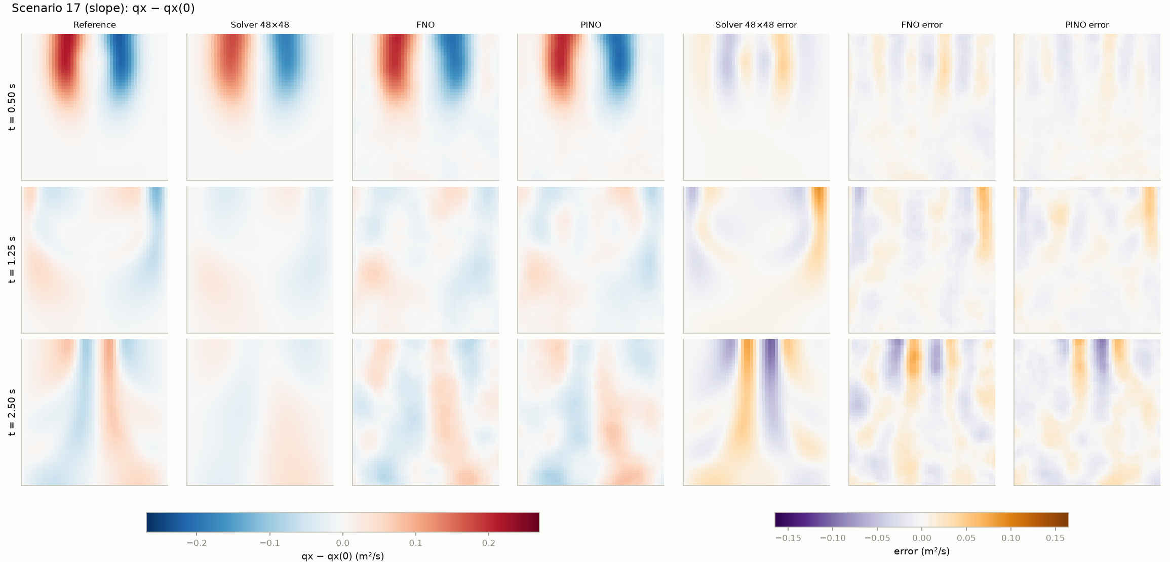
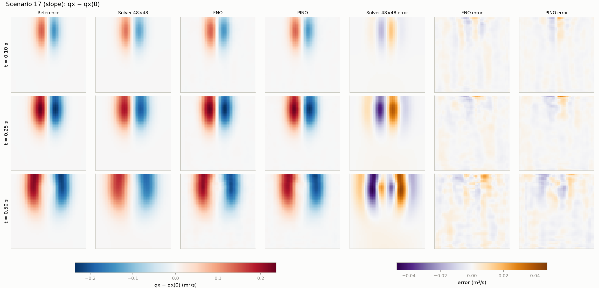
The errors also differ in kind (Figure 5, Figure 6). The first-order solver smooths the waves: its error is large-scale and follows the wave pattern, and it grows as the damping accumulates. The operators keep the waves’ amplitude and position better, but their error is a blotchy, small-scale pattern that does not look like any wave.
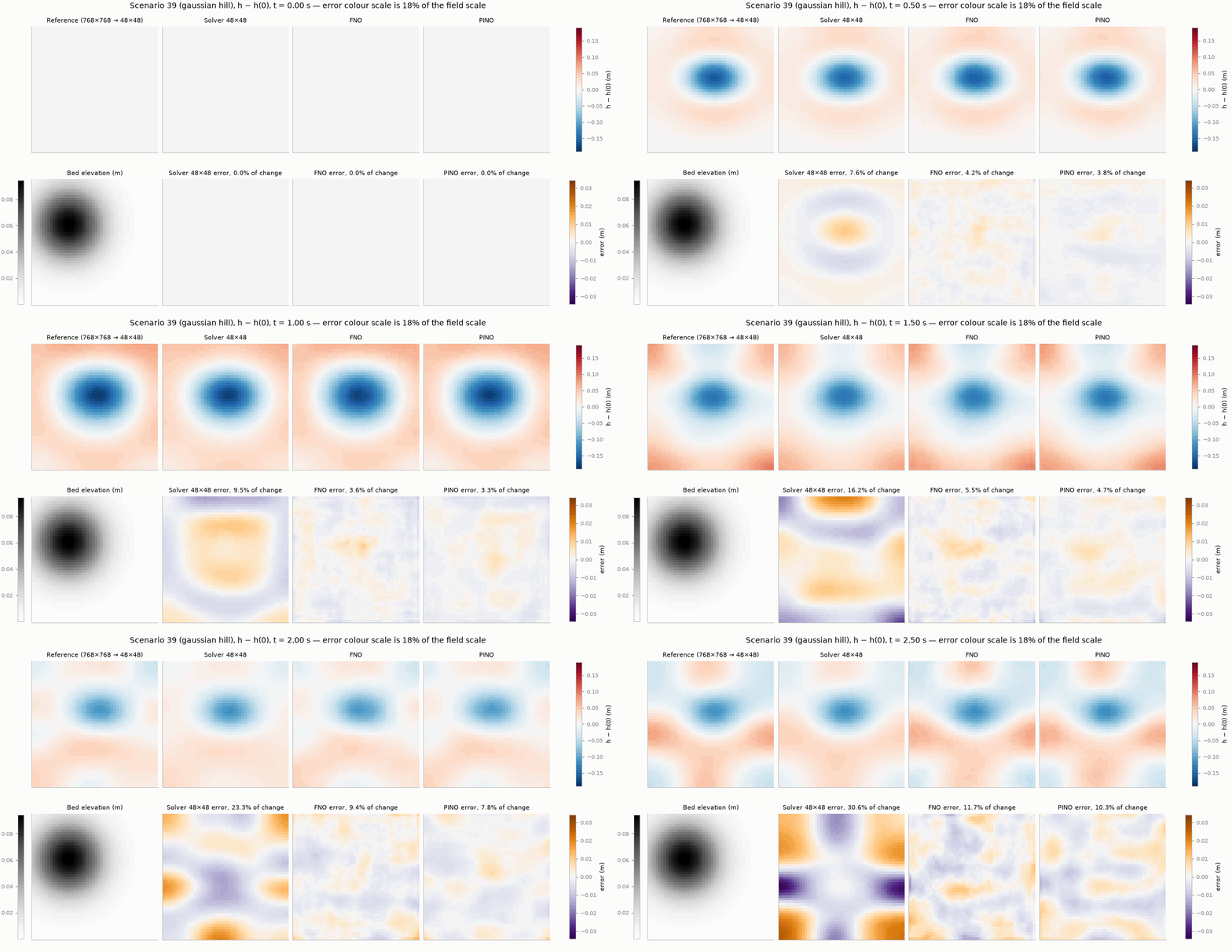
The longer-horizon study is much more expensive than the main one: its data take many hours, and each training run took about 2.5 h on 8 threads, with two running at once.
7 What this emulator is, and is not
It is:
- A demonstration that an operator trained on 56 simulations can predict smooth, fully wet shallow-water flow in unseen scenarios from the same distribution, more accurately than a solver at the same resolution.
- A fair comparison, on identical splits and metrics, of data-only and physics-informed training.
It is not:
- A flood model. There is no wetting and drying, friction, rainfall, inflow, surveyed terrain or field validation.
- Proof of extrapolation. Every test scenario comes from the training distribution. Larger domains, new terrain types and horizons beyond 2.5 s are untested.
- A test of long-time dynamics. The main benchmark lasts 0.5 s, in which waves travel about 2 m in a 10 m basin. The 2.5 s test covers about one basin crossing, with first reflections. Repeated reflections and slow drift over many crossings are untested, and that test uses a single seed.
Summary
- An emulator moves simulation cost offline: train once on solver data, then predict each new scenario in milliseconds.
- Judge it with several metrics: error relative to the change, Equation \(\eqref{eq-skill}\), RMSE, mass error, PDE residual, wall flux and boundary-band error, all on held-out scenarios.
- Here the operators are about 20,000× faster than the reference solver, and more accurate than a solver at the same resolution. A 192 × 192 solver is more accurate still, at about 200× the operators’ cost, so training pays off only after several thousand predictions, Equation \(\eqref{eq-breakeven}\).
- Their accuracy is weaker at early times, on sloping terrain and with few training simulations.
- Over 2.5 s, with reflections from the walls, the operators still beat the coarse solver, by a smaller margin. The physics weight had to be chosen again, and the long-horizon models are less accurate early on than models trained on 0.5 s.
- The benchmark is smooth, fully wet and at most 2.5 s long. Wet/dry fronts, friction, much longer horizons and field data are the obvious next steps, and they are where surrogates are hardest to get right.
Check your understanding
- How much of the 16-fold error reduction comes from the network, and how much from data choices such as symmetry augmentation and refined labels?
- When would you trust an emulator’s prediction for a scenario you have not simulated? What would you monitor?
- Where would physics losses help more: here, or with very few simulations, longer horizons or sparse observations?
- What would change with wet/dry fronts? Think about depth positivity, the residual’s division by \(h\), and the smoothness assumed by Fourier layers.
- Over the first 0.5 s, the models trained on 2.5 s are worse than those trained on 0.5 s. Why? Name two ways to get good accuracy at both early and late times.